This article is by guest author Dimitar Marinov, whom I (Jonas) contacted after seeing his excellent videos about DSP filters. You can read more about Dimitry below the blog post and find a link to his YouTube channel here. But first, read on to learn about verifying digital filter implementations!
This article is part of a series. Click here to read Dimitar’s other articles:
- Part 1: Digital filters in FPGAs
- Part 2: Finite impulse response (FIR) filters
- Part 3: FIR filter types
- Part 5: Polyphase FIR filters
Introduction
So far, the spotlight has fallen over the FIR filter design and its various forms. However, there is a problem that is just as important – how to ensure the implementation is working correctly. Whereas there are some standard techniques, it’s not always clear whether the design is error-proof. Therefore, this post discusses the most essential testing procedures and introduces a verification method that can easily incorporate them.
Impulse Response
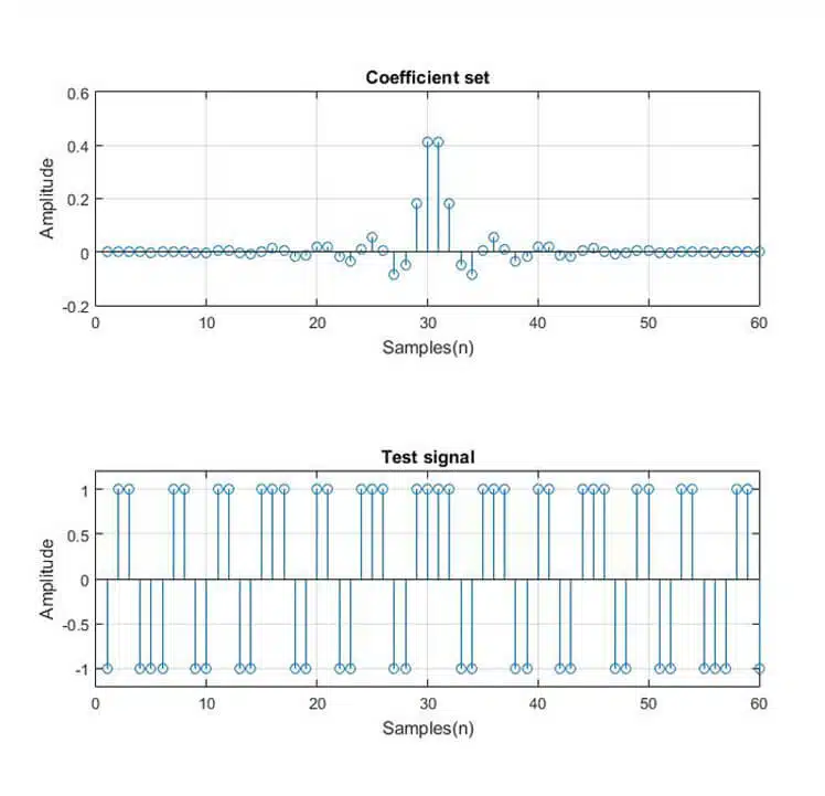
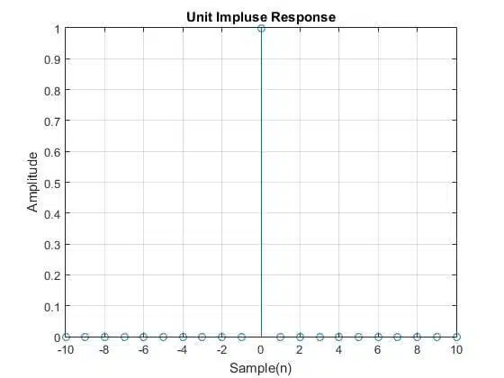
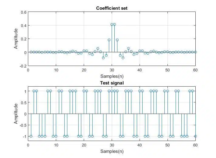
The go-to method of testing FIR filters is to apply a unit impulse response – a unity value followed by zeros, also known as the Dirac delta function (see Figure 1). As the unity value makes its way through the FIR delay line, it passes through every tap, leading to an output that equals the respective coefficient.
Hence, the output sequence contains every filter tap value, ordered from first to last. Here the keyword is tap and not just coefficient since filters, like the previously discussed Half-band and the Shaping Filter, have more taps than coefficient values. The idea behind this test is to compare the output of the filter to the coefficient set or the expected impulse response. Ideally, they should match.
When performing this test, or any others, pipe-lining should be considered as it delays the output, and the result occurs later compared to a non-pipelined implementation. As a rule of thumb, the test should last for at least N+1+P samples after the unit is applied, where N is the number of filter taps and P is the pipe-lining level. This should give enough time for the unit sample to propagate through the whole filter.
What is unity in fixed-point?
When testing the ideal model of the filter, the impulse response has a value of 1.
It is easily applied when evaluating the floating-point implementation, but what about if the data format is fixed-point? In this case, there are multiple answers, but the one that makes sense the most is unity equals one (positive) LSB. Doing so makes sense, as the multiplication product between the coefficient and the unity value would be the coefficient.
Unity equals one LSB*2k
Due to the nature of fixed-point binary arithmetic, the width of the multiplication product equals the sum of the input value widths. If input A is 25-bit wide and input B is 18-bit, product P is 43-bit wide.
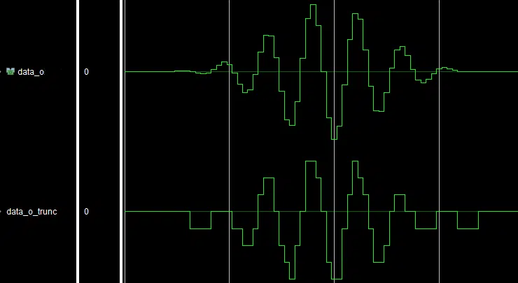
The data growth is not always desired, and to deal with it, the LSBs of the output are rounded or truncated (see Figure 2). In this case, applying an LSB as the unity value will not produce the desired result. This issue can be solved by left-shifting the LSB by the amount of rounded/truncated bits (k).
As mentioned already, the Impulse response test is the most frequently used method to check whether the filter works as expected. Common issues that are detected by this test are:
- Not involving all filter taps in the filtering process – sometimes, the very first/last coefficient can be skipped. Check the filter loop conditions.
- Not multiplying the correct values – make sure all coefficients are correctly indexed by the for loop or counter.
- Not resetting the accumulation register (for serial filters only) – set the accumulation register to ‘0’ when starting/ending the filter loop.
- Having the coefficient set in reverse – is especially important for FIR filters with asymmetric coefficients.
Overall, this is a very comprehensive test, as it can show most of the things that can go wrong during the implementation. If the filter passes this test, chances are it is going to work. The test, however, does not check whether the design is error-proof.
Data Range Test
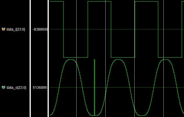
Overflow, and respectively underflow, occurs when the sum of two (or more) binary numbers exceeds the available dynamic range. This is crucial, since the convolution of two vectors requires the sum of multiple products between the input data and the coefficients. Hence, FIR filters are susceptible to overflow/underflow (see Figure 3).
Filter design tools like the FDAtool from MATLAB create coefficients with unity gain in the passband (unless specified otherwise), i.e, there is no amplification of the input and no reason to expect any overflow/underflow. Nevertheless, certain combinations of input and coefficient values can cause errors.
To check whether the design is prone to overflow/underflow, simply sum the absolute values of the coefficient set. If the result exceeds the available value range when there is a change, the output may overflow†.
† Most coefficient sets would exceed the limit, but what also is important is the order of coefficients, i.e., if positive and negative coefficient values alternate, then overflow is less likely.
The idea behind this action is to put the filter in a worst-case scenario where the product of every coefficient multiplication is the absolute value of the coefficient. Such an input would consist only of maximal and minimal values in a specific order.
Whereas the occurrence of such signals is highly unlikely, overflow/underflow can occur in simpler input signals – see Figure 3. In this image, a full-scale square wave is applied to a 60-tap low-pass Equiripple filter. Another example is Figure 5, where the input is a full-scale sine wave. In both cases, errors, represented as spikes, can be observed.
Full-scale signals are rare too, but more likely. Imagine slightly over-driving the input of an ADC – the result is a full-scale signal. Therefore, protecting your design from overflow/underflow is the best way to ensure it behaves as expected.
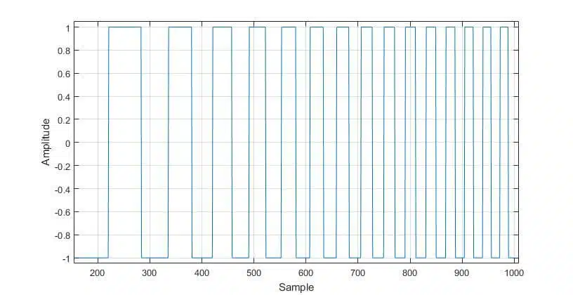
Square wave sweep test
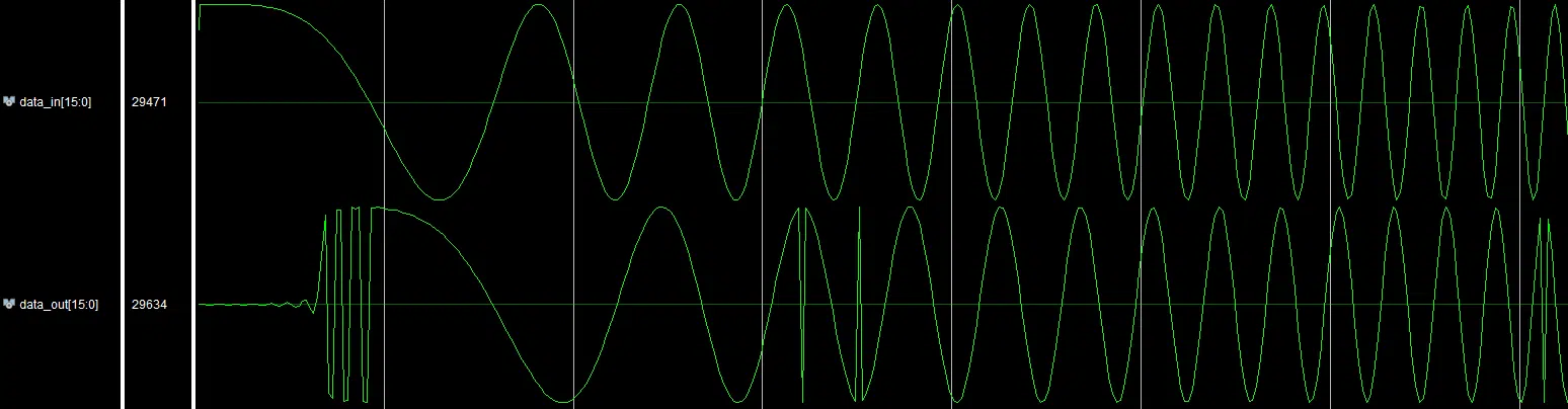
A simple way of testing for overflow/underflow via a square wave sweep that swings between the minimum and the maximum. The idea is to “stress test” the filter by feeding it a signal that contains only the highest/lowest values. That by itself may not be sufficient, which is why it is also important to vary the frequency of the input (see Figure 6), which as a result varies the combinations of min/max values that interact with the coefficient set.
This test is not “bulletproof” i.e. it does not guarantee that an overflow/underflow will be observed. However, it increases the probability of detection. It is fairly simple and can be implemented, and can even be performed with a signal generator and an oscilloscope.
Overflow Mitigation
Gain Correction
There are two ways to handle overflow/underflow error mitigation, and these are gain correction and saturation. Gain correction comes in two flavors – it can be applied to the coefficients or the input data.
- When applied to the coefficient values, the operation can be performed during the design stage. Doing so reduces the need for additional logic. This is achieved by attenuating the coefficient set by a certain factor (discussed later). The operation also impacts the gain of the filter!
- When applied to the input, the scaling must be performed in real-time, requiring one more multiplication. It is possible to implement it as bit-shifting.
The aim of the gain correction is to introduce enough headroom to accommodate the highest possible values. It is also possible to extend the data width of the input signal by adding a couple of bits to the MSBs.
However, the following processes may have to be adjusted to the new data width. This is because any samples that take advantage of the newly added bits cannot be represented with the old data width. As a consequence, this approach may increase the resource use of the design!
The amount of gain correction or MSB bit extension can be found from the absolute sum of the coefficients – in particular, the integer portion of the sum, considering the coefficients range ±1.
Gain \: Correction \: factor = ceil (sum(abs(coefficients)))
MSB \: extension \: factor = floor(sum(abs(coefficients)))
The equations above consider the worst-case scenario. A less strict alternative would be to use the ratio of the expected maximal/minimal sum value (1.3, for example) to the available data range (±1).
Gain \: Correction \: factor = ceil (expected \: max \: sum / data \: range \: max)
MSB \: extension \: factor = floor(expected \: max \: sum / data \: range \: max)
Saturation
Another approach would be to integrate an overflow/underflow correction logic into the design. As mentioned before, the multiplication of two binary values results in doubled data width (see Figure 7). This reflects in both the value and the sign width. Hence, the product has two sign bits of the same state.
Since the sum of the binary numbers is preceded by multiplication, it is possible to take advantage of the sign bits in the following way – whenever an overflow occurs, the sign bits would take different states. This can be used to evaluate whether the sum has overflown (sign bits = “01”) or underflow (sign bits = “10”). Then the value can be corrected accordingly.
The saturation circuit should be applied only when the input values have the same sign. Otherwise, overflow cannot occur. Apart from increased resource use, the negative side of this technique is the impact on the spectral content of the signal, i.e., whenever the signal overflows, it will introduce harmonics that were not there previously whenever the sum saturates.

In most signal processing systems, overflow would result in harmonic distortions. However, In others, it can lead to severe consequences. One such case is the Ariane flight V88, where due to speed vector overflow, the self-destruct mechanism of the rocket was triggered, which led to a loss of more than $370 million USD[1, 2].
Despite the overflow occurrence of the given example is of a different nature, it is important to consider the effects the overflow can have on the system. FIR filter can also be used to “take decisions”. Such is the application of the Matched filter, which correlates the input to a predefined kernel[3]. The output of the filter is the similarity between the input and the coefficient set. Overflow in this application can lead to false/missed correlation events.
HDL Co-simulation
The previously discussed testing methods can be implemented in various ways, with the most obvious being a self-checking HDL test bench. The main issue with that is the amount of effort needed to develop the testing environment.
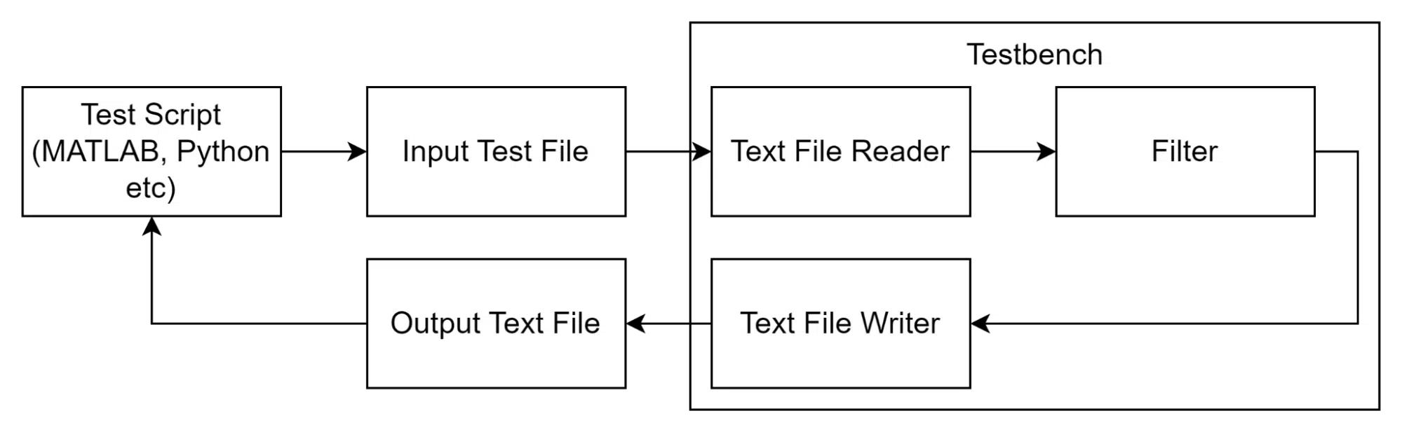
An alternative to this approach is a software-based co-simulation, where a script is used to generate the test bench stimuli and analyze the output. In this case, the HDL test bench serves as a text file interface, where the input data is read from the script-generated file, and the result is written to a separate text file.
Text IO
VHDL can communicate with external programs by reading and writing files, most commonly text files (.txt). This is achieved with the textio libraries that contain the necessary functions. The library can work with bit vectors and hexadecimal values. However, the integer data type is the better choice for this application because it is easiest to use across various languages. Moreover, this avoids the conversion from integer to binary or hex in the software script, which saves some work.
Reference Modelling
In the script, the user can generate any type of test stimuli – impulse response, step response sine sweep, etc. The key feature of this approach, however, is the ability to compare the performance of the HDL filter with a reference design, i.e., the same filter but implemented in software.
The reference model can implement an ideal version of the filter (i.e., floating point) or a bit-accurate that takes into consideration the arithmetic operations on a binary level. For the latter option, it is important to consider every binary process – saturation, truncation, rounding, etc. Otherwise, the model may not match the performance of the HDL implementation.
The reference modeling approach can be used for other algorithms and more complex signal paths as well. In the references, there is a Matlab script and a VHDL test bench that evaluate the performance of a 60-tap Equiripple FIR filter. The script also calculates the absolute sum of the coefficient set.
Improvements
Currently, the script is not “aware” of the HDL testing environment. Therefore, it is required to start the simulator manually and run the simulation whenever the stimuli are generated. The whole workflow can be automated via Tcl – the software script can generate a Tcl script that opens the simulator and then runs it until the test is over.
Other testing techniques
Step Response
There are other ways to test your design: step response and sweep response. The former can be recreated with the square wave sweep whenever the period of the square wave is at least two times longer than the filter length in samples. That is, if the filter is 60 taps, then the period should be 120 samples or more. It can also be used for overflow/underflow checking; however, I found that a square-wave sweep does a better job.
Sweep Response
The sweep response is also useful – it can be used to validate the frequency response of the filter. To achieve this, a sine wave sweep is applied to the input, and the output of the filter is transformed into a frequency domain. Then, the values of each measurement are superimposed.
This test makes more sense once the design is implemented and running on the hardware, i.e., it can be used to validate the filter’s performance. One thing to consider is the sweep time – it would be much longer than the FFT window. Otherwise, the frequency plot will not be that accurate. Alternatively, the measurement can be done with white noise instead of a sine sweep; however, the result is not as precise.