Part 3: FIR filter types

This article is by guest author Dimitar Marinov, whom I (Jonas) got in touch with after seeing his excellent videos about DSP filters. You can read more about Dimitry and find a link to his YouTube channel below the blog post. But first, read on to learn about digital filters in FPGAs!

This article is part of a series. Click here to read Dimitar’s other articles:

Introduction

The previously discussed filter describes a general-purpose device that can fit in many applications but is not necessarily the optimal solution. This is where application-specific FIR structures come in. Therefore, this post aims to present some of the more popular filter structures used in specialized applications.

Mean average

In many statistical applications, it is desirable to find the average of an input. We can do this with an FIR filter. If all of the coefficients are equal to ‘1’, the output will result in the sum of all values stored in the delay line. On the other hand, if all coefficients are equal to 1/N, where N is the number of filter taps, then the output equals the mean average of all values stored in the delay line. Since all coefficients are the same, we can rearrange the structure of the filter as such:

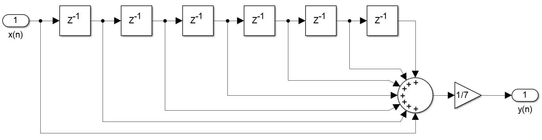
**Figure 1:** 7-tap MA filter with common coefficient

This is a surprisingly useful device as we can use it for low-pass filtering, noise reduction, statistical applications, etc. It acts as a low-pass filter whose response is determined by the number of filter taps [1]. If the number of filter taps = 2k, where k is an arbitrary integer, then the coefficient(s) can be implemented as a bit-shifting operation.

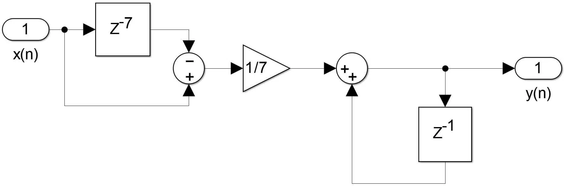
There exists another version of the filter, called recursive moving averager – it reduces the number of operations to an addition, a subtraction, and a multiplication (see Figure 2). Notice the Recursive Mean Averager has N delay elements, whereas the non-recursive has N-1.

Folded FIR filter

Very often, the FIR filter coefficients are symmetric around the middle value. This property can be exploited, thus reducing the multiplication operations by a factor of ~2 [2].

**Figure 3:** Plot of 10th order symmetric FIR filter coefficients

This is achieved by applying the mathematical identity property to the convolution algorithm, where:

y(n) = c(1)*x(n) + c(2)*x(n-1) + c(3)*x(n-2) + c(4)*x(n-3) + c(5)*x(n-4) \texttt{ where } c(1) = c(5) \texttt{ and } c(2 ) = c(4)

Equation 1: Convolution with 5 elements example

y(n) = c(1)*(x(n) + x(n-4)) + c(2)*(x(n-1) + x(n-3)) + c(3)*x(n-2)

Equation 2: Rearranged convolution example

If x is the input data and c is the coefficient set, then from Equation 2, it can be seen that before the multiplication, the respective elements from the delay line have to be summed (i.e., pre-added). Summing, however, can lead to overflow/underflow if the values are too high/low due to bit growth. This can be avoided by dividing the input by 2 and multiplying the output by 2 [3].

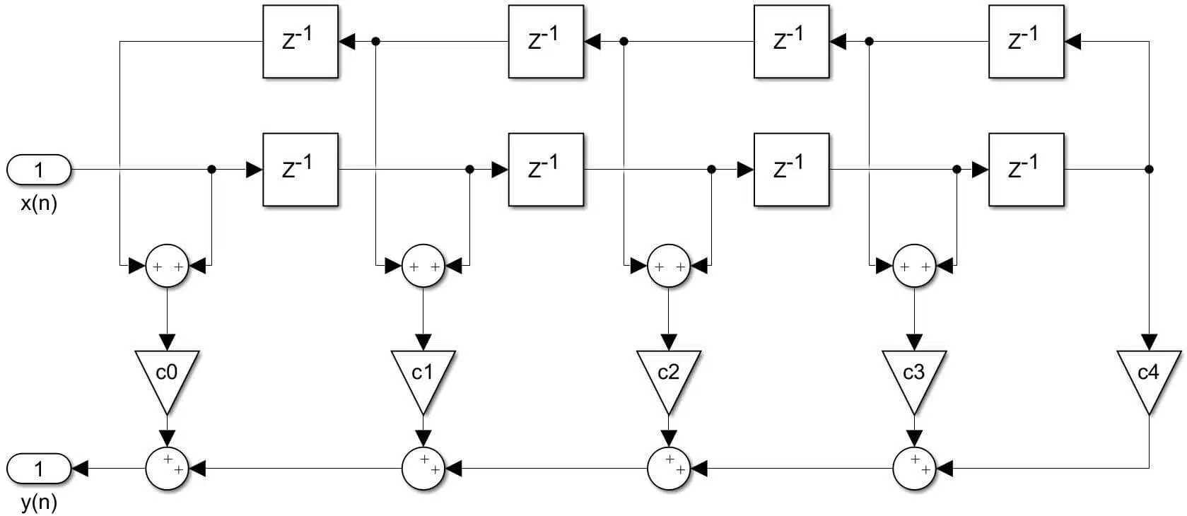
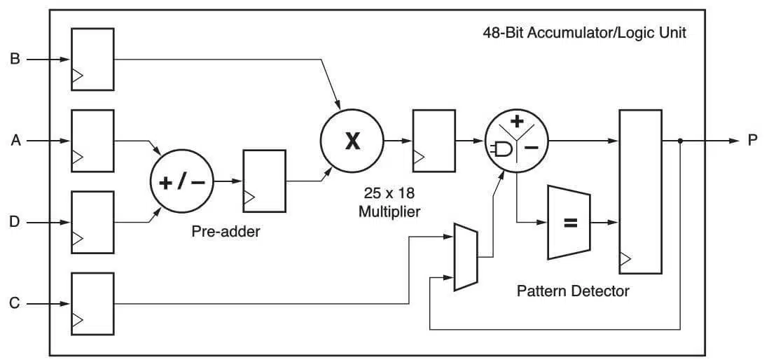
**Figure 4:** 8th order Folded FIR filter

Figure 4 presents a 9-tap folded FIR structure – notice that the amount of multiplications is reduced, whereas the amount of delay elements remains the same. Also, the structure differs for odd and even tap filters. Some arithmetic units like DSP48E1 (see Figure 5) have embedded pre-adders, thus further reducing the cost of the implementation.

**Figure 5:** DSP slice available in Xilinx’s 7 series devices

Half-band FIR (and other bands)

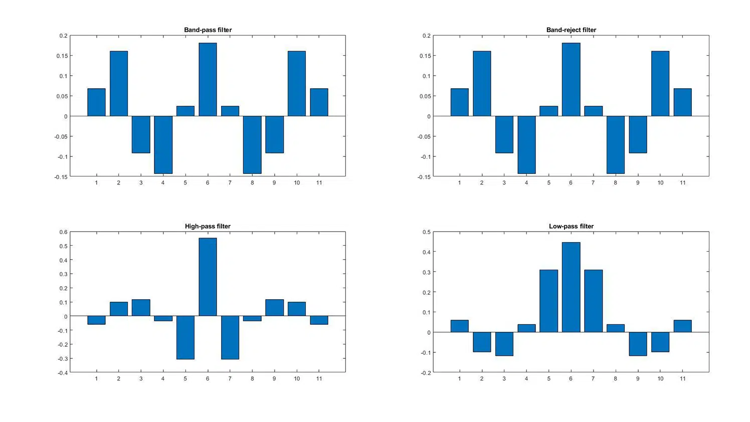
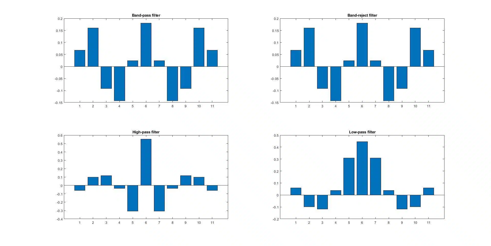
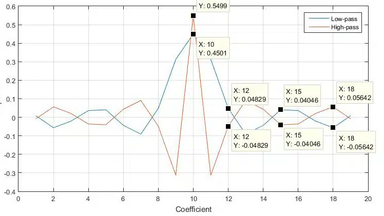
Another technique that exploits the filter coefficient properties is the half-band filter. It has been observed that many filter design methods produce filter coefficient sets containing a lot of zeros when the filter is low-pass or high-pass and the cut-off frequency (Fc) is Fs/4.

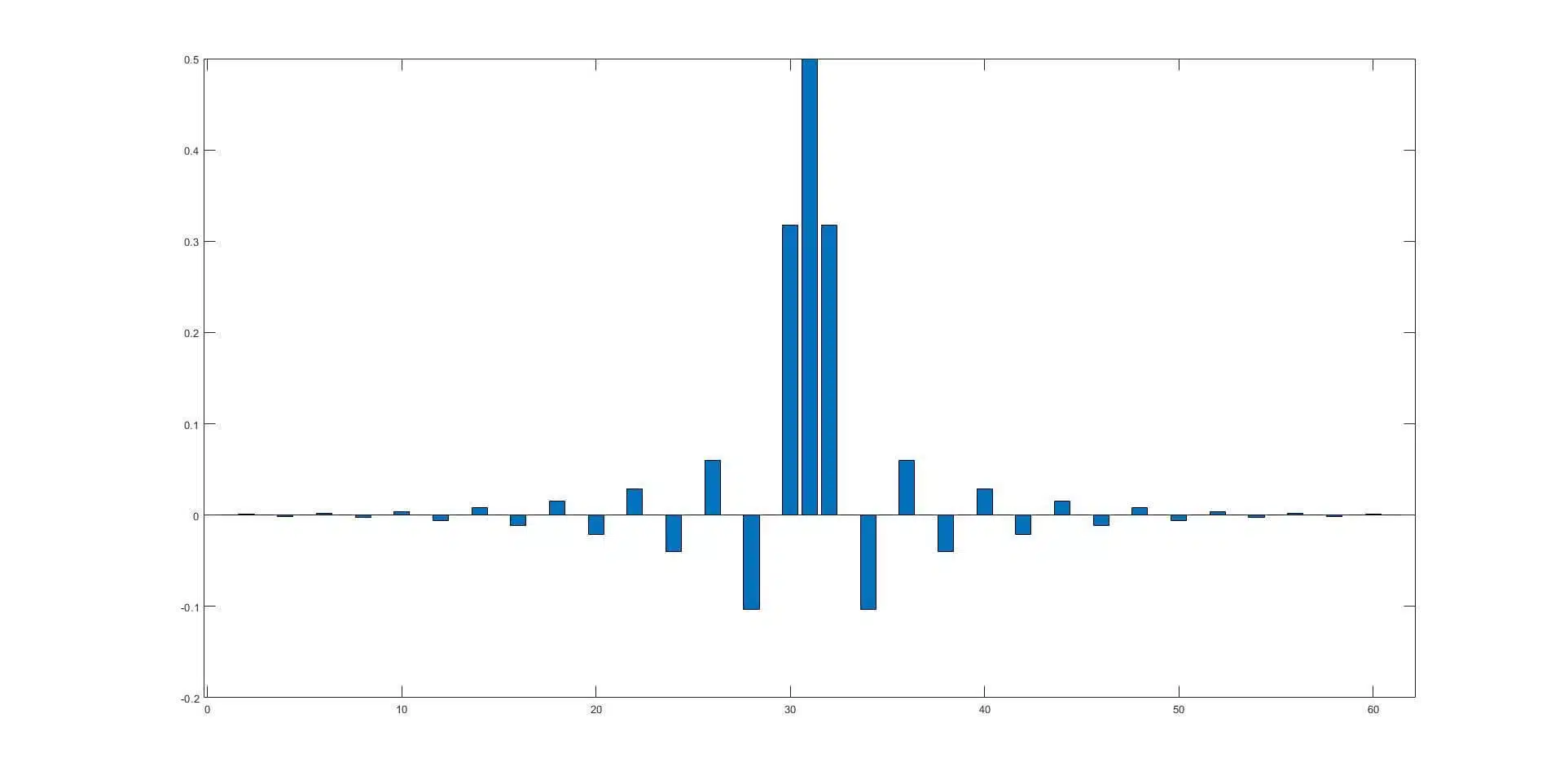
**Figure 6:** 60th order Half-band low-pass Hamming filter coefficients

Moreover, the zero-values coefficients tend to alternate with the non-zero valued coefficients (see Figure 6). This allows for reduction of the multiplication operations by removing all multiplications by 0.

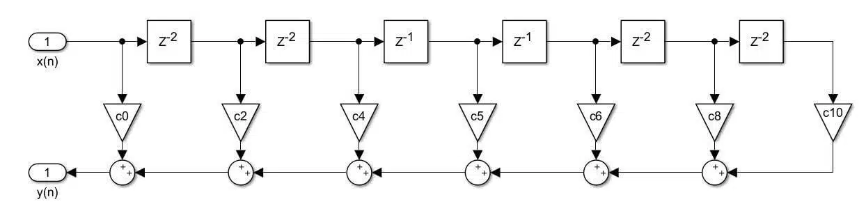
**Figure 7:** 10th order Half-band FIR filter structure

A suggested Half-band FIR filter structure is shown in Figure 7, where there are only 6 multipliers instead of 11, and some of the delay elements are doubled. It is also important to mention that this filter structure can be used only with coefficient sets that have an odd amount of coefficients (even order).

The half-band idea can be expanded to other ratios of Fs-to-Fc. For example, having Fc = Fs/6 results in ~⅓ of the coefficients being zeros, and Fc = Fs/8 has ~¼ of the coefficient values being 0.

Complementary FIR filters

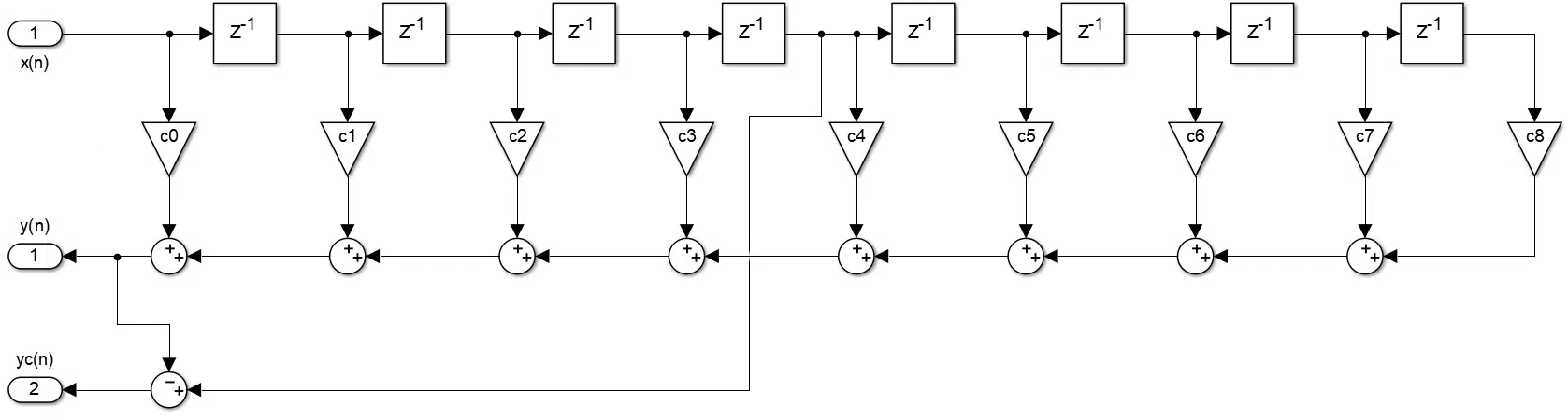
Two functions are said to be complementary when the sum equals unity. Filters also implement a function, and with slight modification, a regular FIR filter can output the complement of the original function. I.e., if the filter is low-pass, then the complement would be a high-pass (see Figure 8, where y(n) is the direct function, and yc(n) is the complementary function).

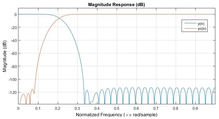
**Figure 8:** Example of complementary filter output frequency response (60th order)

To achieve that, we subtract the output of the filter from the sample located at the middle of the delay line (see Figure 9). This technique finds use in filter-bank decomposition, where Half-band filters are used to split the spectrum into low and high frequencies. One must remember that we can only use this structure with even order filters.

Polyphase FIR filters

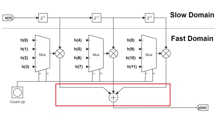
This class of filters is used explicitly in sample-rate conversion. Typically, FIR filters have a single delay line running from the input to the output, Polyphase filters, however, have multiple delay lines running in parallel (see Figure 10 and Figure 11). We can easily conclude that the structure is composed of several parallel sub-filters.

However, it must be noted that the filter coefficients are shared between the sub-filters. I.e., the coefficients are split into phases, hence the name of the filter. Another unique feature of the Polyphase filters is the multiplexer used to switch between the sub-filters.

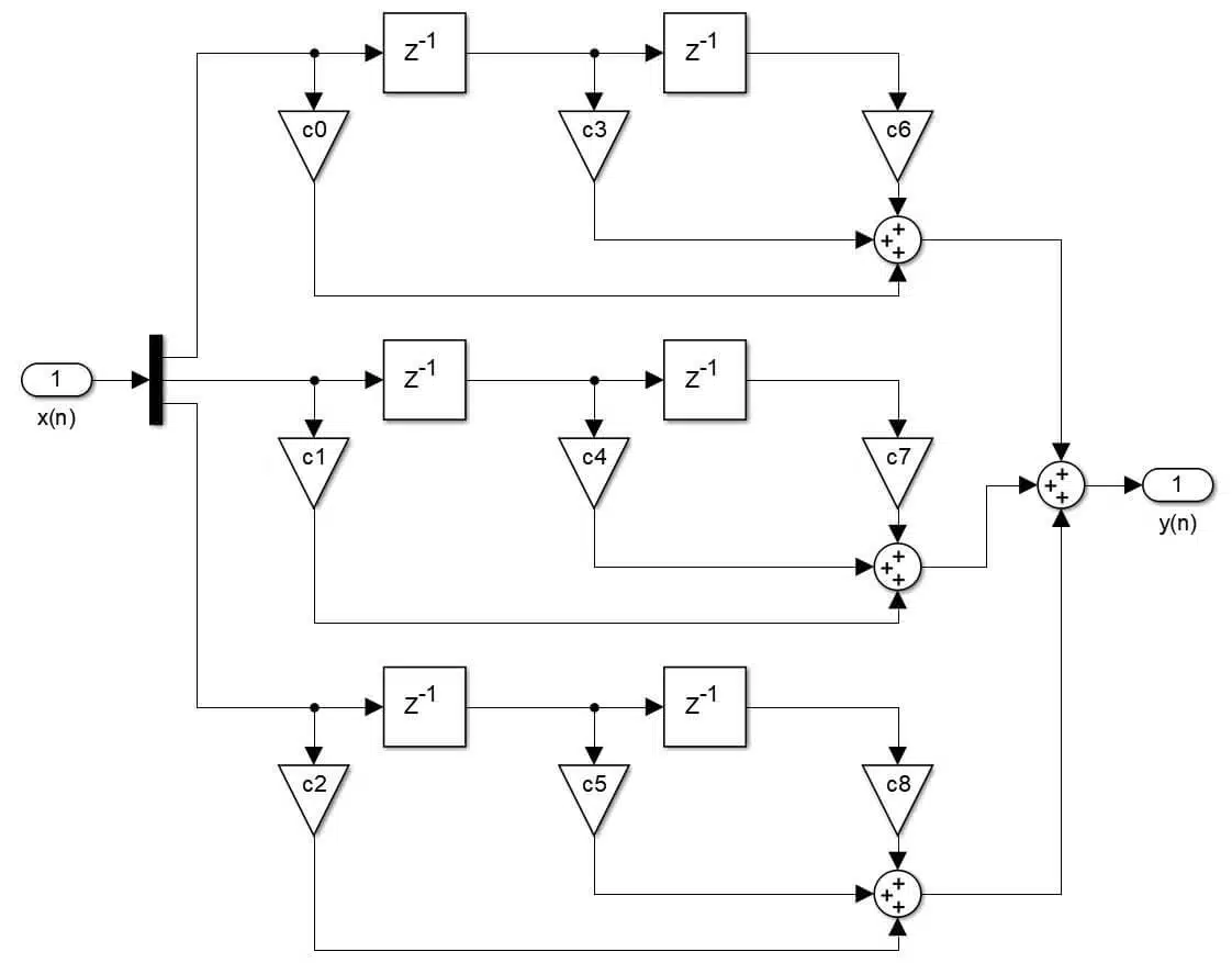
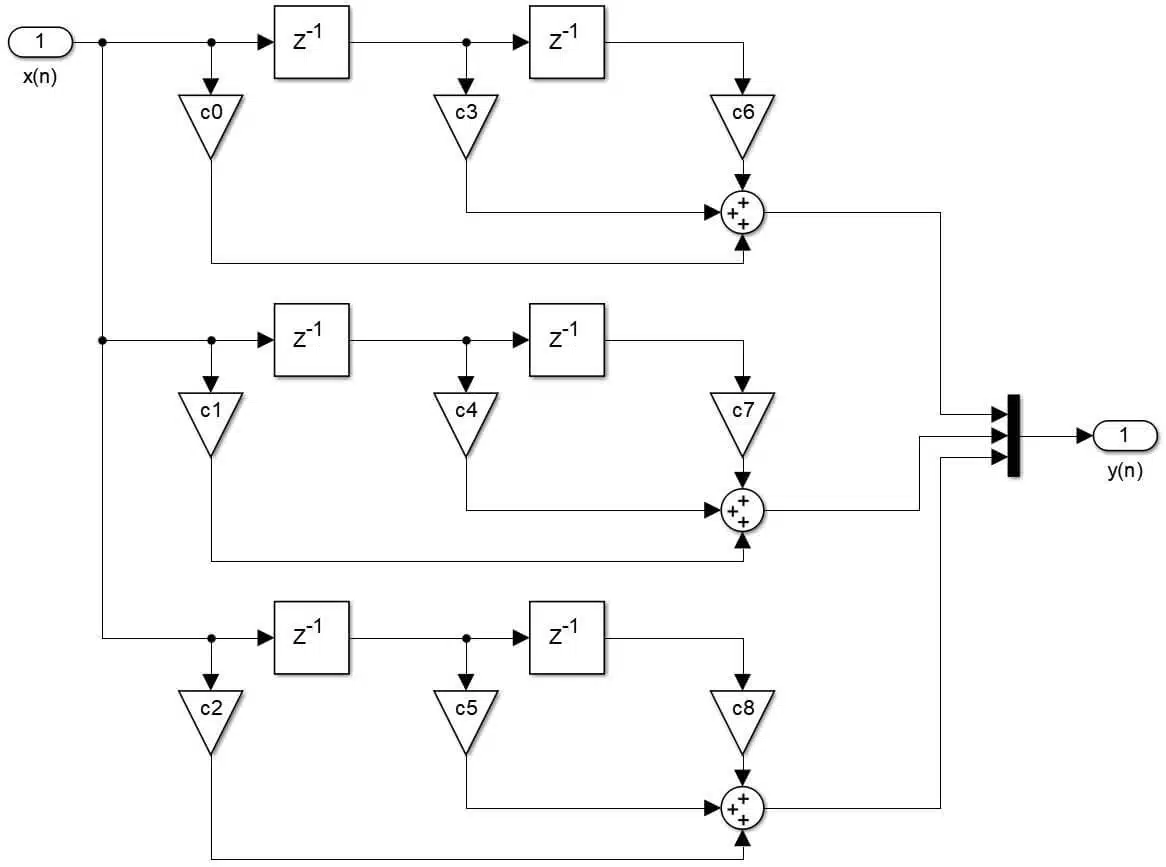
**Figure 10:** Polyphase filter for decimation

**Figure 11:** Polyphase filter for interpolation

Sampling-rate conversion, the process of changing the sampling frequency, consists of two stages – sample inserting/discarding and filtering, where the filtering is always performed in the faster domain. Polyphase filters combine the two stages, and as a result, the filter operates at a slower sample rate, which leads to an overall computational load reduction.

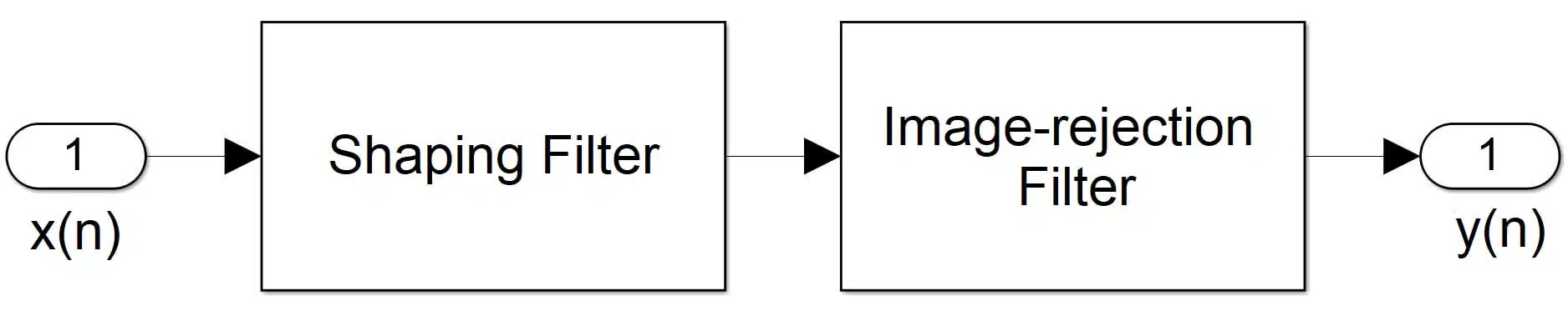
Interpolated FIR filters

This structure combines two filters to create a device highly optimized for narrow-band filtering. It consists of a shaping filter followed by an image reject filter.

**Figure 12:** Block diagram of an Interpolated FIR filter

The shaping filter is based on a direct FIR, but what makes it different is the delay line – instead of having one delay element per tap, it has multiple. I.e., the filter delay line is expanded by a factor of M (see Figure 13).

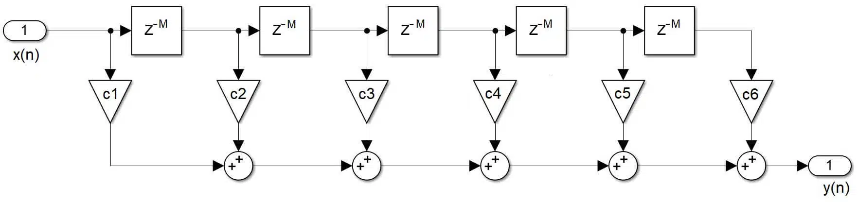
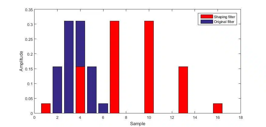
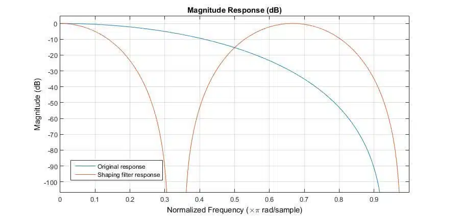
**Figure 13:** Block diagram of 15th order shaping filter

This extends the filter output by inserting zeros between the samples (see Figure 14) and compresses the spectrum M times. As a result, spectral images of the filter pass-band appear across the whole frequency range (see Figure 15).

**Figure 14:** Impulse responses of a prototype filter (original) and the respective shaping filter

This is where the second filter comes in – it removes the unnecessary frequencies by filling the zeros, i.e., it interpolates the output of the shaping filter, which is where the structure’s name originates. The image-rejection filter is a regular FIR filter. Keep in mind that the interpolated filter does not interpolate the signal, i.e., there is no change in the sampling rate.

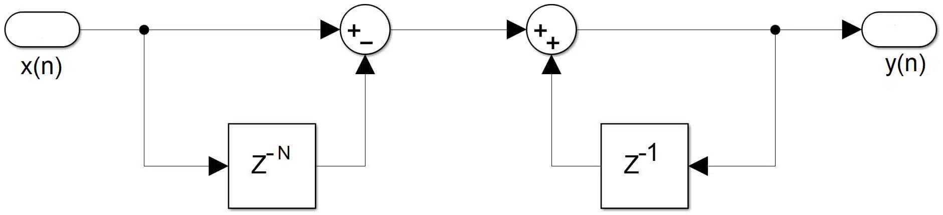
**Figure 15:** Frequency responses of a prototype filter (original) and the respective (compressed) shaping filter

Cascaded integrator-comb (CIC) filters

As the name suggests, this structure is composed of two cascaded filters – a comb filter and an integrator.

CIC block diagram - a comb (left) followed by an integrator (right) — **Figure 16:** CIC block diagram – a comb (left) followed by an integrator (right)

Most commonly, the CIC filter is used in combination with other filters, especially in sampling-rate conversion applications. Doing so relaxes the performance requirements of the other filter(s) and hence the resource use.

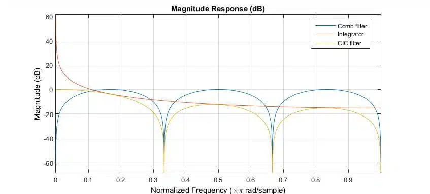
Note: The magnitude of the filters has been normalized. We achieved that by applying the following coefficients: 0.5, 0.34, and N for comb, integrator, and CIC, respectively.

Comb

This filter is based on the idea of phase cancellation; hence the frequency response is directly determined by the length of the delay line (see Figure 18).

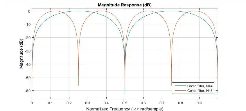
As a result, the spectrum (0Hz to Fs) gets divided into N-amount of peaks, separated by deep notches resembling a hair comb hence the name. At first glance, this device does not look very useful. However, it is very handy when dealing with spectral images. The idea is to locate the notches of the filter at parts of the spectrum where the spectral images lie.

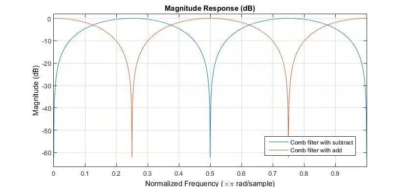
By changing the subtract operation to an addition, the location of the notches switches their place with the location of the peaks (see Figure 19). This, however, disrupts the CIC frequency response. Apart from CIC, comb filters are also used in audio applications as sound effects.

Frequency response of a comb filter hen subtracting/summing the delay line — Figure 19: Frequency response of a comb filter when subtracting/summing the delay line

Integrator

Similar to the comb, but with feedback, this device realizes a low-pass filter aiming to attenuate the upper part of the spectrum. The filter, however, has very high gain at low frequencies and DC, which can easily lead to overflow/underflow caused by the feedback. A recommended solution is to extend the data width of the signal.

Sharpened FIR filters

This technique can be used to “sharpen” the frequency of an already-existing filter. If the order or coefficients of a filter cannot be changed, then one way to improve the frequency response of the filter is by cascading – this doubles the stop-band attenuation, but also the pass-band ripples.

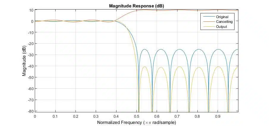
**Figure 20:** Frequency response comparison

To avoid the drawbacks of the simple filter cascade, one can use Sharpened filters – a method that can improve the stop-band without worsening the pass-band (see Figure 20). It also relies on cascading. However, it uses a copy of the filter to create a complementary signal that is used to cancel out the undesired effects of the cascaded response (see Figure 21).

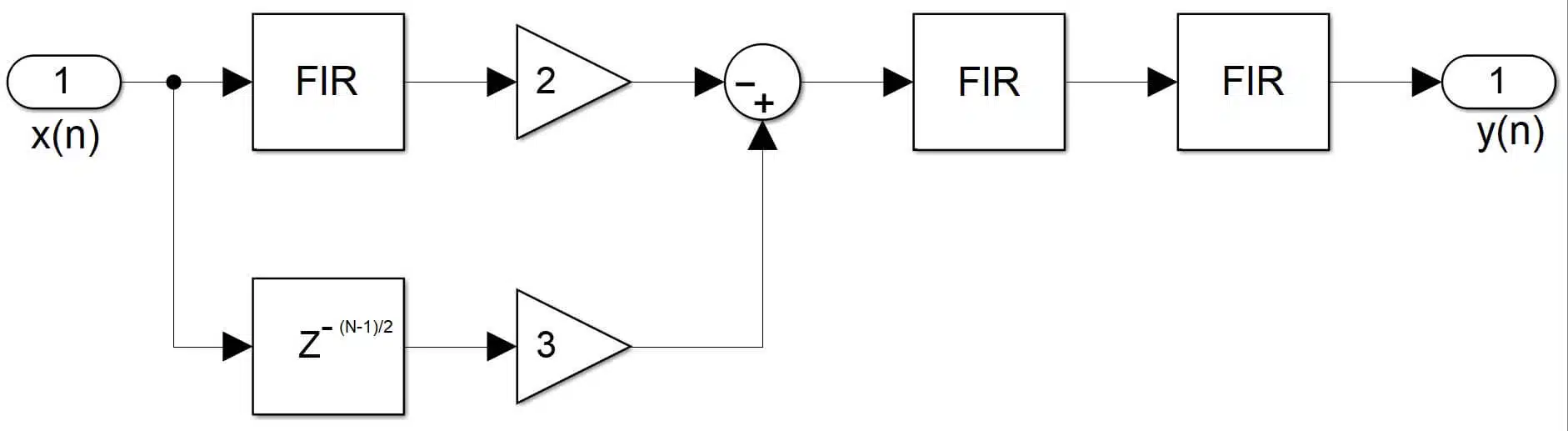
**Figure 21:** Sharpened filter block diagram

Since the structure employs a delay line to generate the complementary response, the following limitations apply to this method:

Using an FIR filter with a linear phase in this technique is essential. This is because the delay line, used to derive the canceling response, acts as a linear-phase element. Therefore, this method cannot be used with minimum-phase FIR filters and IIR filters. Otherwise, the phase relationship between the signals going through the first filter and the delay line is disrupted.
The order of the filter must be even (odd taps). This is because the delay line must equal the filter’s group delay, which is derived from the following formula, where N is the number of filter taps:

\textit{Group delay }G = (N-1)/ 2

Another thing to consider is the susceptibility to overflow – To prevent this, the filter coefficients must have unity gain.

Other FIR filters

Hilbert transformer

Most filters are designed to modify the frequency response of an input. Some applications, however, require phase adjustment without any amplitude modification, and in very specialized applications, it is desirable to have an exact phase difference of 90 degrees. To achieve this, a device called Hilber Transformer is used – an FIR filter with carefully designed coefficients.

The coefficients of odd-taps Hilbert Transformers have the same property as the Half-band filters, making them favorable for use with the Half-band filter structure. Have in mind that despite being an all-pass filter, the FIR Hilbert Transformer does attenuate part of the spectrum.

Matched FIR filter (correlation)

Typical filters use a set of coefficients that aim to modify the input’s phase and spectrum. Usually, these coefficients are the output of filter design algorithms.

Matched filters, however, use time-domain data as the coefficient set. In this case, the filter is used to correlate the input data to the coefficients, i.e., it is looking for the presence of the predefined sequence. In this case, the output will indicate the correlation – the higher the output, the more similar the data is to the coefficient set.

When it comes to implementation for this application, the most likely choice is the normal FIR or the folded FIR, depending on the coefficients set. Matched filters are commonly used in distance measurement (LIDAR, RADER, SONAR) and digital communications.

Minimum phase

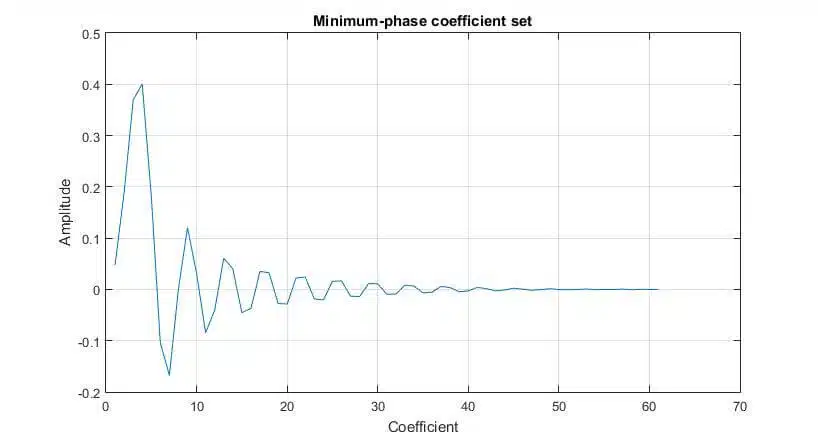
Since most filter coefficients are symmetrical, it takes a while for the output to develop – this is called group delay, and it equals (N-1)/2. Here, N is the number of taps. However, for some applications, it is required to have a fast response, which is incompatible with the filter’s group delay.

One way to avoid this is by designing a Minimum-phase filter. That is an FIR filter whose impulse response is not symmetric – instead, it is designed to minimize group delay by placing higher-valued coefficients first along the delay line. This, however, comes at the cost of a non-linear phase response. Having non-symmetrical coefficients implies that Minimum-phase filters cannot make use only of the direct and transposed FIR filter structures.

**Figure 22:** Minimum-phase coefficient set

Part 4: FIR filter testing

Click the link below to view the next article in this series!

Part 4: FIR filter testing

References

[1] Richard G. Lyons, “11.5 Filtering Aspects of Time-Domain Averaging” in Understanding Digital Signal Processing
[2] Richard G. Lyons, “13.7 Simplified FIR Filter Structures” in Understanding Digital Signal Processing
[3] Applying this technique will introduce errors – the exact impact depends on the data and coefficient widths as well as their values. Depending on the application, these errors can be ignored.