This article is by guest author Dimitar Marinov, whom I (Jonas) contacted after seeing his excellent videos about DSP filters. You can read more about Dimitry below the blog post and find a link to his YouTube channel here. But first, read on to learn about complementary finite impulse response (FIR) filters!
This article is part of a series. Click here to read Dimitar’s other articles:
- Part 1: Digital filters in FPGAs
- Part 2: Finite impulse response (FIR) filters
- Part 3: FIR filter types
- Part 4: FIR filter testing
- Part 5: Polyphase FIR filters
Introduction
Complementary filters refer to a group of filters whose frequency response sums up to unity, i.e. their collective responses form an all-pass filter. When the complementary system is composed of only two sub-filters, let’s say filter A and B, it is possible to omit one of the filters (B) and derive its output from the difference between the system input and the output of filter A (also called a prototype filter).
This scheme is also referred to as complementary filters and is particularly useful for FIR filter design, leading to multiply-accumulate (MAC) operation reduction by a factor ~2.

Complementary FIR Filters
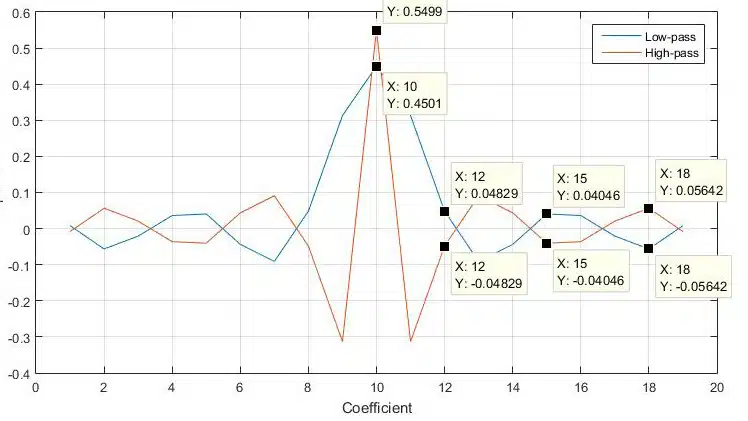
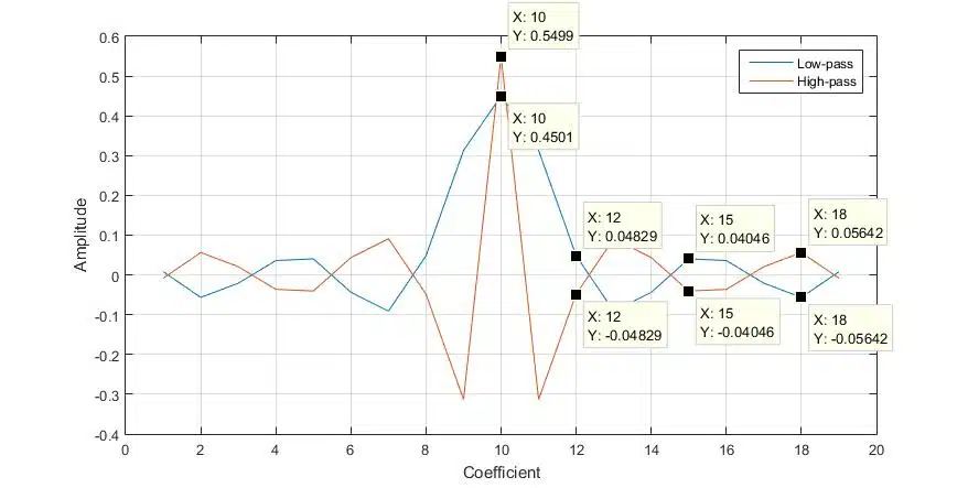
The reason this works, with odd-tap liner-phase FIR filters in particular, is hidden in the coefficient set. It can be observed (see Figure 3) that for this type of filter, the power complementary coefficient pair is almost identical, with two key differences:
- The middle coefficient value from filter B equals 1 – middle coefficient value from filter S set.
- All other coefficient values are equal in magnitude but opposite in amplitude.
This “symmetrical” property is valid only for odd-tap linear phase low-pass, high-pass, band-pass, band-stop, and multi-band FIR filters.
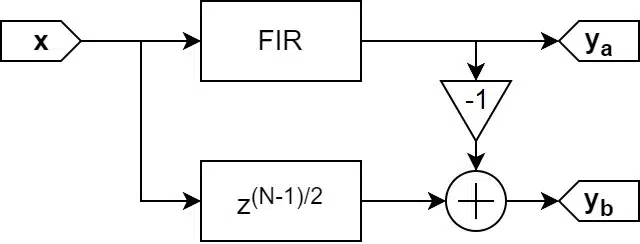
Since it is possible to obtain the FIR filter coefficients by applying an impulse response, following the logic of phase cancellation, it would be possible to obtain the power complementary filter coefficients by subtracting the output of the prototype filter from a copy of the input. This would invert the coefficient sign.
To obtain the middle value, however, the impulse response copy has to be aligned with the middle filter coefficient. This is done by delaying the input signal copy by (N-1)/2 samples, where N is the amount of prototype filter taps. This delay is also known as the FIR filter group delay [SDSP, p9]. The implementation can be verified by comparing the impulse response of the two outputs.
Notch Filter
It is also possible to use the complementary filter scheme to create a Notch filter. To achieve this, the output from the prototype filter has to be scaled by 2.

The centre frequency of the notch is located at the -6dB point of the sub-filter frequency response. This works for any response type, i.e. low-pass, high-pass etc. If the prototype filter is a band-pass or multi-band filter, then there would be a notch at any point the frequency response crosses the -6dB point (see Figure 5).

Here are some of the observations on the response of the derived “complementary” notch filter.
- The notch attenuation is not infinite. Attenuation depends on multiple factors – design method, filter order, cut-off frequency etc.
- Notch filter slopes are proportional to the prototype filter slope and the filter order, respectively.
- The derived notch response has worse pass-band response – the pass-band ripple magnitude is approximately doubled (see the responses in Figure 4).
- The desired response is achieved only at this particular gain value, i.e. the prototype file must have unity gain.
Limitations
Filter Phase and Order
The above-discussed coefficient property is critical for the successful implementation of the complementary pair. Even-tap filter coefficients, however, do not possess this quality, and hence, they are not suitable for this application. Minimum-phase FIR filter and infinite impulse response (IIR) filter are also unsuitable due to their non-linear phase behaviour. Having that said, this technique may work with linear-phase even-tap FIR or non-linear phase filters as well; however, it is unlikely to produce a power complementary pair.
Filter Gain
Another factor that can impact the complementary filter performance is the filter gain. It can be presented as a value that scales the filter coefficients. If the coefficients are scaled, then the middle coefficient of the complementary filter would not compute correctly, which in return would modify the frequency response of the complementary filter. Therefore, the filter must have unity gain (see Figure 6).

Filter Cut-off Frequency
The symmetrical property of the coefficients described earlier is most evident when the cut-off frequency is at the half-band (Fs/4). As the cut-off deviates from the half-band frequency, the symmetry between the complementary coefficient pair is disrupted, resulting in altered performance, most notably in the pass-band and stop-band characteristics of the filter (see Figure 6).
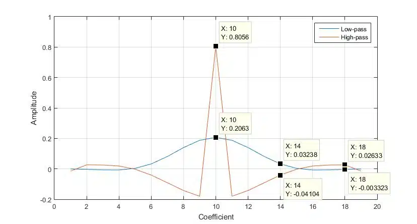
As it can be seen in Figure 7, the symmetry between the prototype (Low-pass) and the reference (High-pass) coefficient sets is disrupted. As a consequence, the complementary filter response derived from this prototype would not sum up to an all-pass filter. Luckily, not all filter design methods perform the same, hence some designs are less susceptible to the coefficient symmetry degradation – Equiripple and most window methods seem to perform much better than Constrained Equiripple.
Complementary IIR filter structures
The complementary filter technique can also be applied to IIR filters as well but with limited success. The Complementary IIR Filters are made of all-pass IIR filter blocks with different phase responses, resulting in phase cancellation or amplification of frequency components in different parts of the spectrum. Creating high-performance complementary IIR filters, however, is not as simple as the linear-phase FIR filters. [4], [5].
Applications
Complementary Filters find use in various applications:
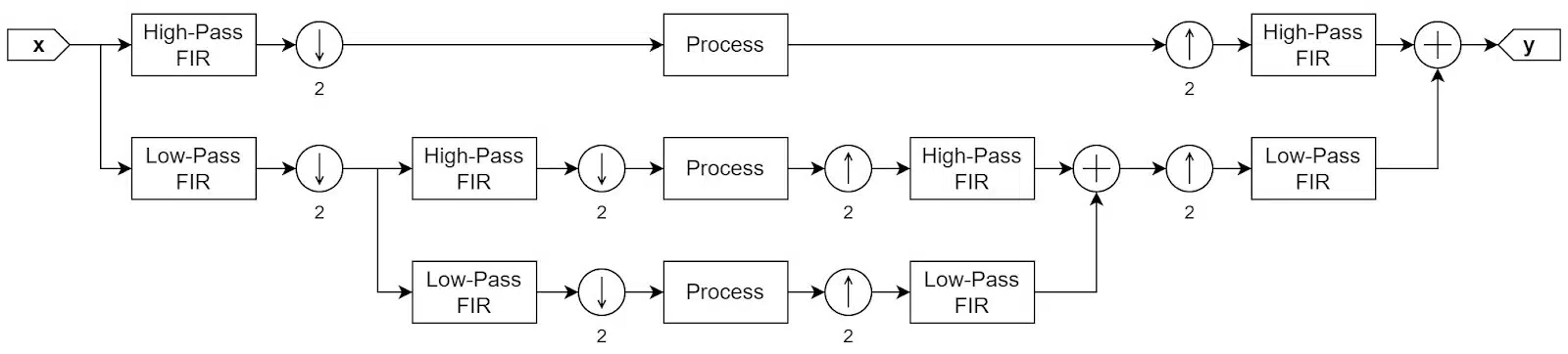
- Multi-rate Filter Banks: Cascades of complementary filters, followed by upsampling and downsampling, can be combined to implement filter banks for signal deconstruction and reconstruction (see Figure 8). These devices find multiple applications such as Wavelet Transform [6], Compression etc.
- Control Systems: The complementary filters can be used to split the sensor data drift from the actual measurements or isolate high-frequency data variations that contaminate a slowly varying measurement [7], [8].
- Audio Processing: Splitting an audio signal into multiple bands gives greater control over the signal content and expands the processing techniques that can be applied to the input [9]. In some application, like Loudspeaker Crossover [10], splitting the signal into multiple bands is essential for success implementation.
- Noise reduction in video (Coring): in this application, it is assumed the noise is high-frequency. A complementary filter is used to extract the noise, which is then being evaluated [11].
Implementation
Transversal FIR Filters
If the FIR filter is implemented in a Direct form (transversal), where the delay elements are before the multipliers, it is possible to omit the additional delay line. Instead, the input signal would be taken from the middle tap of the delay line, thus further reducing the resource requirements of the scheme.
As mentioned before, the Transversal FIR filter structure is not suitable for parallel filter implementation on FPGA due to the summing operations after the coefficient multiplication. Therefore, in this design, only Transposed FIR is considered. As a consequence, the input data would require a separate delay line.
Delay Line Implementation
There are multiple ways to design a delay line. However, when it comes to code complexity, the choice is between a simple register array and a RAM-based implementation. The former is more suitable for lower-order filters (less than 64), whereas the latter is more suitable for higher-order filters. The RAM implementation would require additional logic to move the read/write pointers.
A suitable candidate for this application would be a FIFO, an IP that may be available from the vendor library. For this implementation, however, it has been decided to proceed with the register array. Apart from the code simplicity, it is easier to scale the array implementation so it fits the filter order (i.e. parameterize it via a generic).
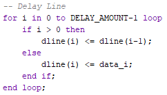
When it comes to the array code, all that is needed is an array declaration and a for loop in a clocked process.

Subtract Operation
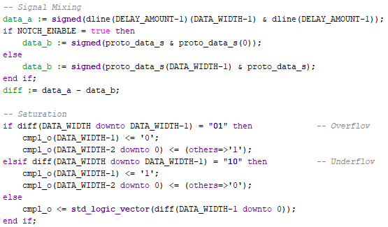
To derive the complementary output, the prototype filter output is subtracted from the delay line output. This operation is susceptible to underflow. Therefore, a saturation logic is added after the subtraction to mitigate the error.
The two values are expanded by adding an extra MSB to the vector with the same state as the current MSB (i.e. adding a second sign bit). In case of an overflow or an underflow, the difference between the two values would have sign bits with different states. Depending on the two MSB values, it can be observed what the error is – whether an overflow or an underflow.
- MSB = “01”: the difference has overflown.
- MSB = ”10”: the difference has underflown.
The Notch implementation does not require two additional MSBs – it has been noticed that adding a single MSB would not cause issues, even though the prototype filter output is multiplied by 2 (left-shifted by one bit.).
The prototype filter, the delay line, and the summing operation are placed in a container whose diagram corresponds to Figure 2 and 4.
Testing
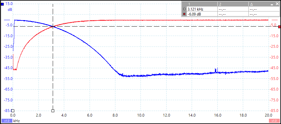
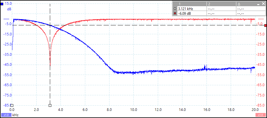
To validate the design, a simple test setup is implemented – the complementary filter is embedded into an audio signal chain operating at 96kHz (see Figure 13). The filter uses a 40th-order Chebyshev low-pass filter with a cut-off frequency of 3kHz. The performance analysis of the filter is realized via a signal generator and a spectrum analyzer.

Despite the sampling frequency, the analysis window covers the spectral window between 100Hz and 20kHz; hence, the signal generator creates a sine-wave chirp within the covered range.
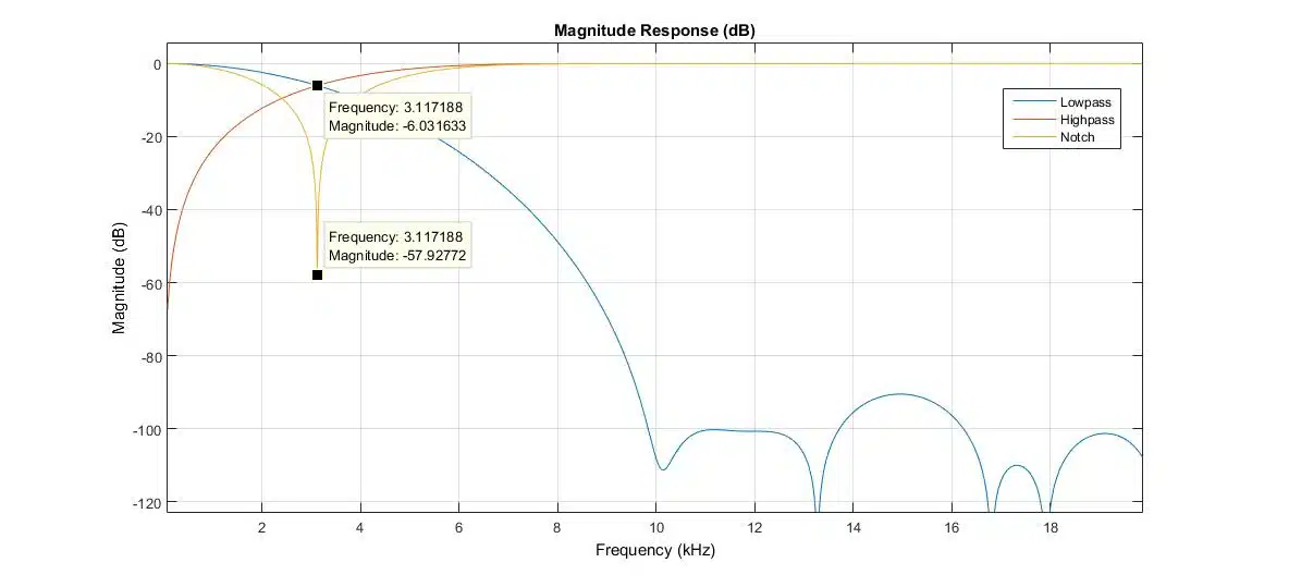
The expected performance can be seen in Figure 14, where the quantized response of the filters is displayed. The crossover point of -6dB is at ~3kHz. There also lies the centre of the derived notch filter, which provides ~58dB of attenuation.
As it can be seen from the measurements (see Figure 15 and 16), the design performance is very similar to the reference – the cut-off point matches closely. The overall shape of the response is also similar to the reference. One exception is the stop-band of the implementation – it does not go below -100dBs. This could be due to the presence of noise in the measurement signal.
References
- [1] Source code
- [2] “Lost Knowledge Refound: Sharpened FIR Filters” from Streamlining Digital Signal Processing, Richard G. Lyons.
- [3] On power-complementary FIR filters, P. Vaidyanathan
- [4] A class of complementary IIR filters, H. Johansson; T. Saramaki
- [5] Three classes of IIR complementary filter pairs with an adjustable crossover frequency, L. Milic; T. Saramaki
- [6] Multirate Filter Banks from Wavelet Analysis and Its Applications, Bruce W. Suter
- [7] Kalman filter vs. Complementary filter
- [8] A_comparison_of_complementary_and_kalman_filtering.pdf
- [9] Multi-band Processing & Distortion, Craig Anderton, Sound On Sound, August 2011
- [10] Audio crossover, Wikipedia
- [11] Chapter 31 “Video signal processing” from Digital Video and HD (Second Edition), Charles Poynton