Part 5: Polyphase FIR filters

This article is by guest author Dimitar Marinov, whom I (Jonas) contacted after seeing his excellent videos about DSP filters. You can read more about Dimitry below the blog post and find a link to his YouTube channel here. But first, read on to learn about polyphase finite impulse response (FIR) filters!

This article is part of a series. Click here to read Dimitar’s other articles:

• Part 1: Digital filters in FPGAs
• Part 2: Finite impulse response (FIR) filters
• Part 3: FIR filter types
• Part 4: FIR filter testing

Intro

Polyphase filters are a class of specialized filters used in sample rate conversion. Whereas most FIR filters have one delay line, Polyphase filters have multiple. To understand the logic behind this, we’ll first have to dive into the topic of sample rate conversion.

Sample Rate Conversion

Sampling rate conversion is the process of changing the sampling rate of a given signal. It comes in two flavors:

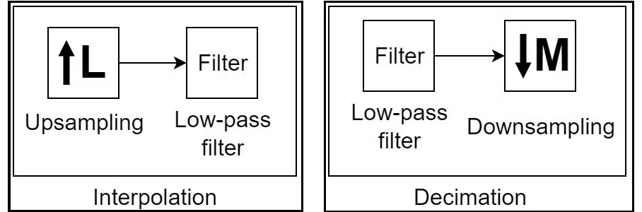
• Interpolation: increasing the sampling rate by a factor of L
• Decimation: decreasing the sampling rate by a factor of M

Up-sampling and down-sampling

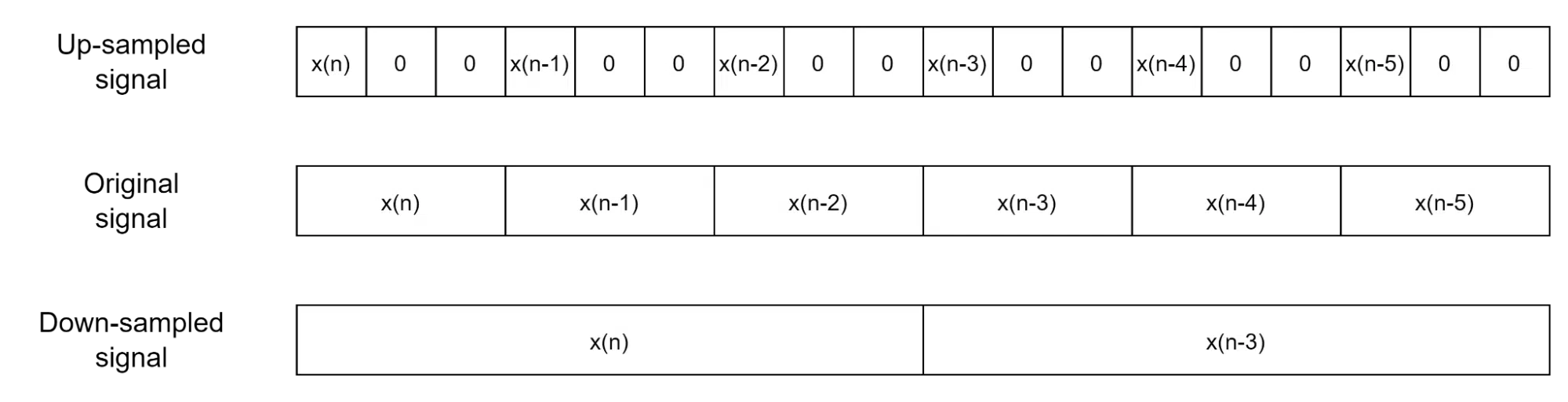
Interpolation is achieved by decreasing the period of the existing samples and inserting zero-value samples to fill in the gaps. This process is called up-sampling. Similarly, during decimation, a certain number of samples are discarded periodically. The period of the ones that remain is extended. This is the process of down-sampling.

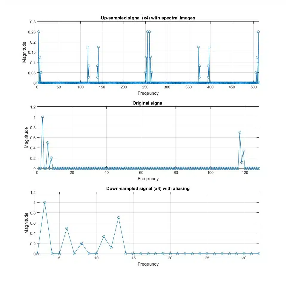
Aliasing and Spectral Images

These two operations, however, come with side effects. The up-sampling process creates copies of the signal across the new spectrum, i.e., spectral images. The down-sampling operation, on the other hand, shifts all high-frequency components that cannot be represented with the new sampling rate into the lower part of the spectrum. This is called aliasing.

Filtering

To remove the undesired side effects, the signal needs to be filtered. For interpolation, the signal needs to be filtered after the up-sampling, where it has to remove the spectral images. In decimation, the filter is applied before the down-sampling process to remove all components that would alias into the new passband. This makes interpolation and decimation two-stage processes.

This post focuses on the implementation aspects of Polyphase filters. To get a deeper grasp of the theory behind the sample-rate conversion and how to design such a system, check [1].

Polyphase Filters

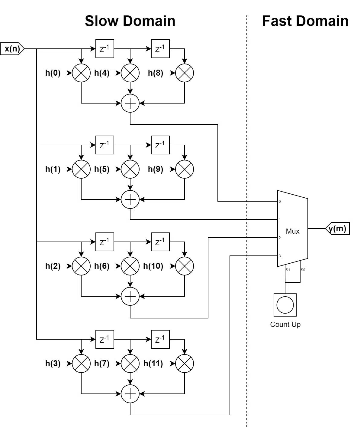
Polyphase Interpolator

The sampling rate conversion, as described above, is quite computationally inefficient. In the case of interpolation, the filter has to perform numerous operations on zero-valued input samples. These operations can be skipped. The operations with the zeros are avoided by splitting the filter into L sub-filters, also called phases, hence the name of the filter.

The data is fed in at the slow data rate, and the output of each phase is multiplexed at the higher sampling rate. This technique relies on the fact that after the up-sampling process, the original samples are “separated” by a fixed number of zeros. Hence, it is possible to predict which operations are required to calculate the output as the data propagates through the delay line.

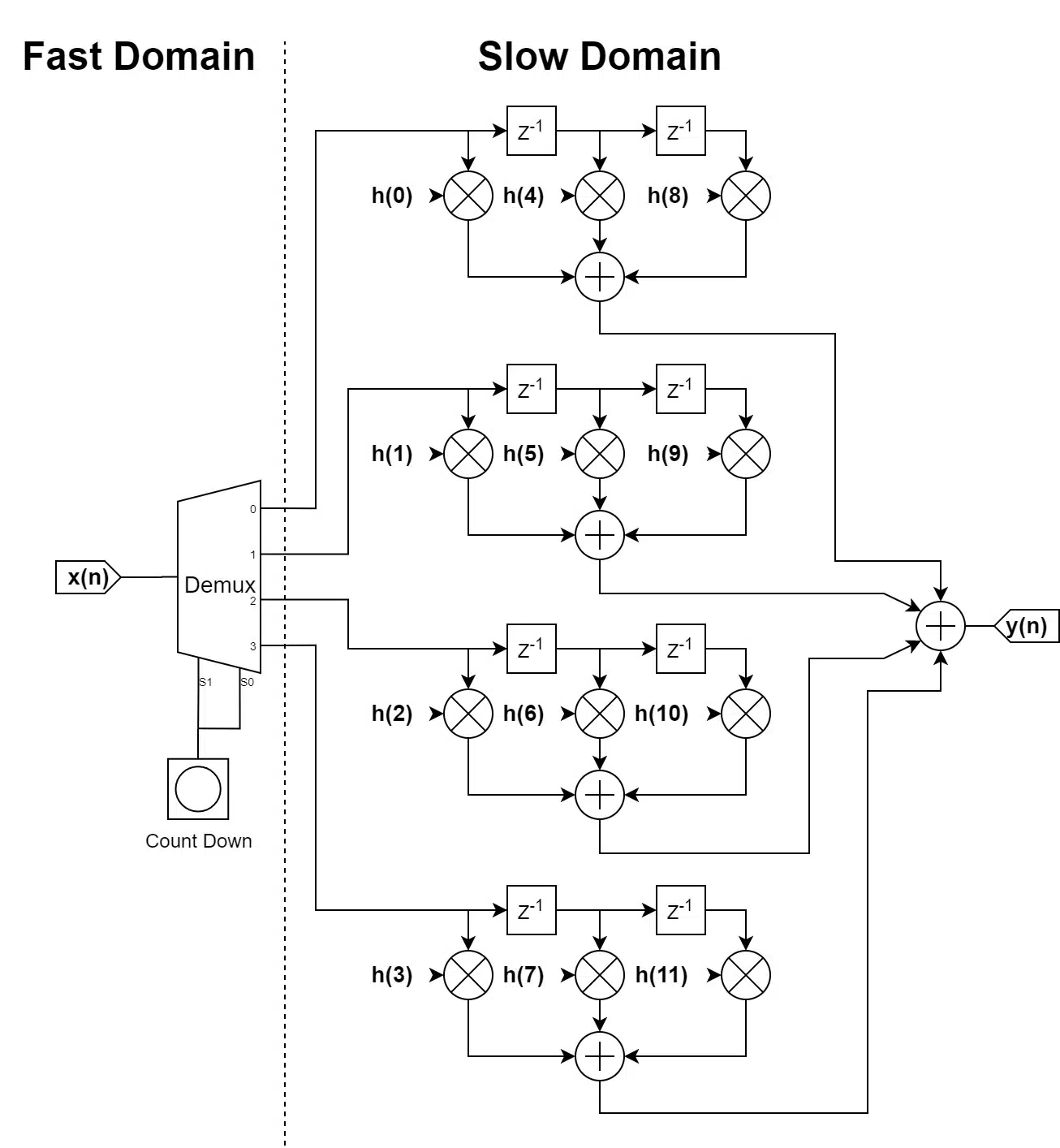
Polyphase Decimator

The decimation process has a similar issue – most of the filtered samples are discarded by the down-sampling stage. Hence, the same approach is applied to the Decimation process, but “in reverse”. Since the down-sampling process discards samples periodically, it is possible to “enable” the filter only when an output has to be produced.

To be precise, the data is shifted along the delay line all the time; however, the actual convolution is performed only when necessary. In other words, the convolution is performed on blocks of the input samples. This property is used to split the filter into M phases and multiplex the incoming data between them. The data arrives at a fast sampling rate, but as soon as asserted to the sub-filter, it is processed at a slower sampling rate.

Filter Optimization

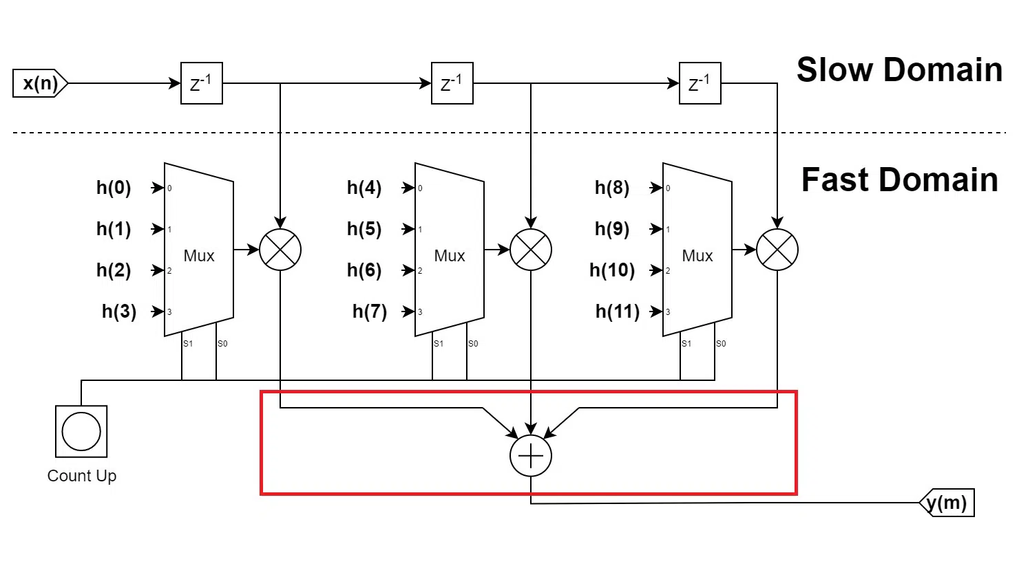
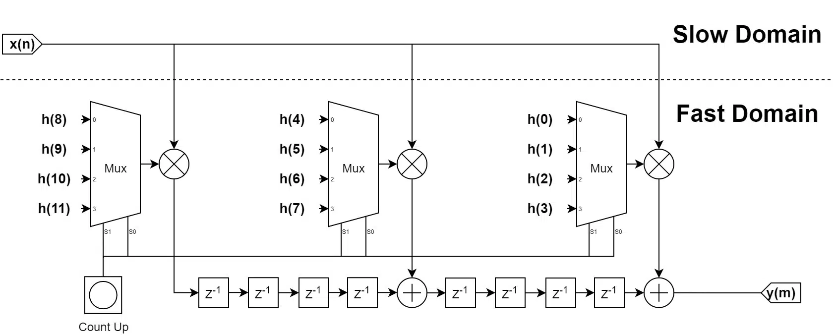
As it can be seen from the block diagrams of the filters, these architectures are not that efficient when it comes to resource use. In fact, they use the same number of multipliers. The only benefit is processing the data in the slow domain. When it comes to the Polyphase Interpolator, it is possible to improve the resource use by rearranging the filter structure so the coefficients are multiplexed instead of the sub-filters. This works because all phases receive the same input data.

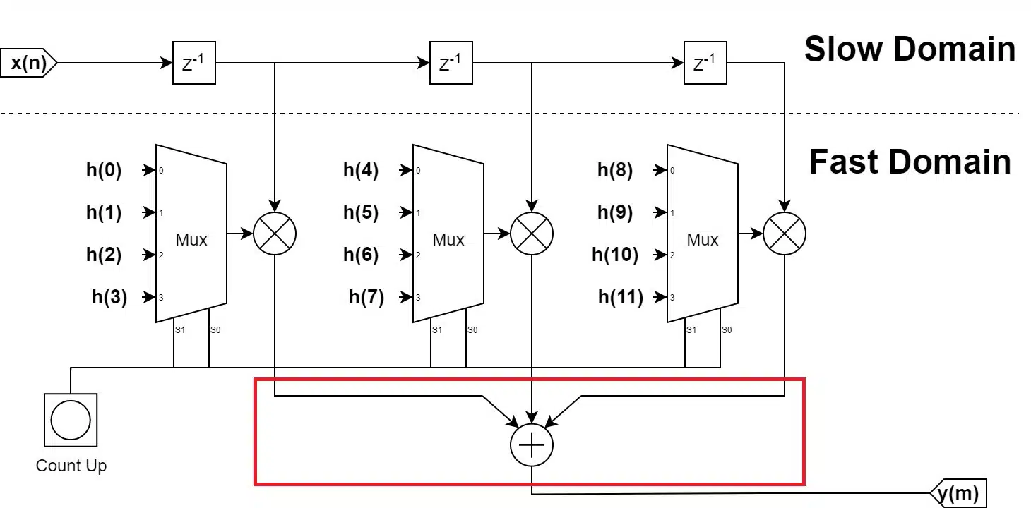
The structure comes with some disadvantages, in particular, the signal path between the delay line registers and the output – the path can become too long and hence cause timing issues. This can be avoided by transposing the filter, i.e., moving the delay line after the multipliers. Since the delay line is moved in the fast domain, it has to be adjusted accordingly.

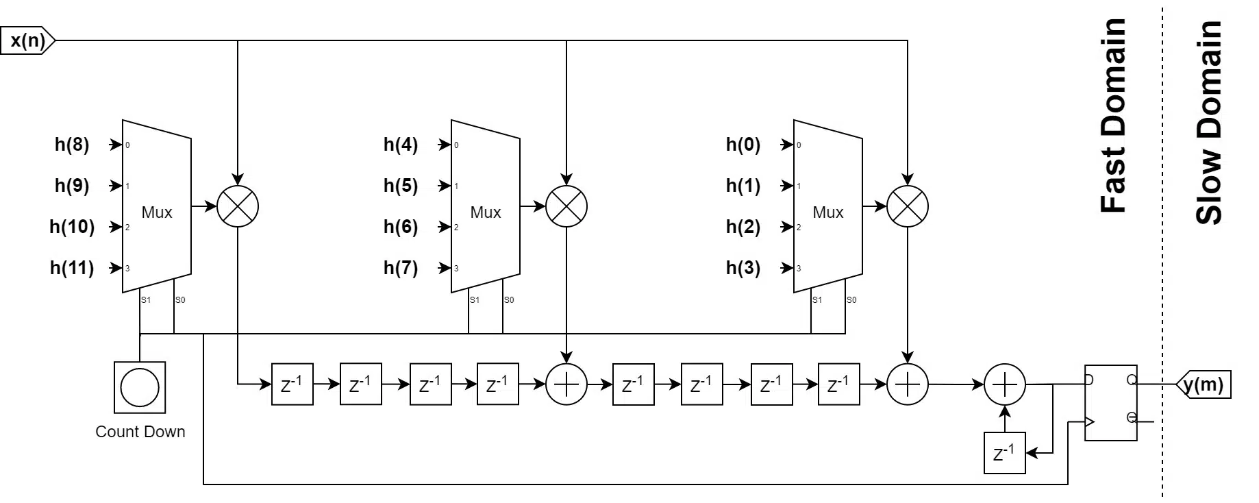
The same filter structure can be applied to the Polyphase Decimator, except that an accumulator is required to sum every M samples to produce the final output.

A demonstration code combining both filters into one can be found in the references [2].

Alternative Implementations

A polyphase filter for decimation and interpolation is proposed by Xilinx in UG193 [3] (Figure 4-30 and Figure 4-31). The filter structures are optimized for the Xilinx architecture, and hence it is expected to achieve better timing performance. Despite the document being applicable for Virtex 5, it is also relevant for the 7-series FPGAs since the DSP architecture is almost identical.

As demonstrated already, it is possible to implement the Polyphase Interpolation filter by adding a latching register at the input of the Decimation Filter. The same can be applied to the Xilinx interpolation filter too. Hence, the main difference between the Xilinx version and the one derived in the previous section is the location of the delay line – in the Xilinx version it is at the input of the DSP slices.

Because there are pipeline registers between the DSP slices, one more delay register is added to each delay segment. As a result, an offset has to be added to the filter coefficient index. This implies the Xilinx filter would be a bit more difficult to implement – it has to have L coefficient index counters, each with a different offset.

Interpolated FIR Filter

Not to be mistaken with the Interpolation FIR filter discussed in the previous section, this filter is used to create very narrow low-pass filters. It is actually composed of two filter stages (also called sub-filters):
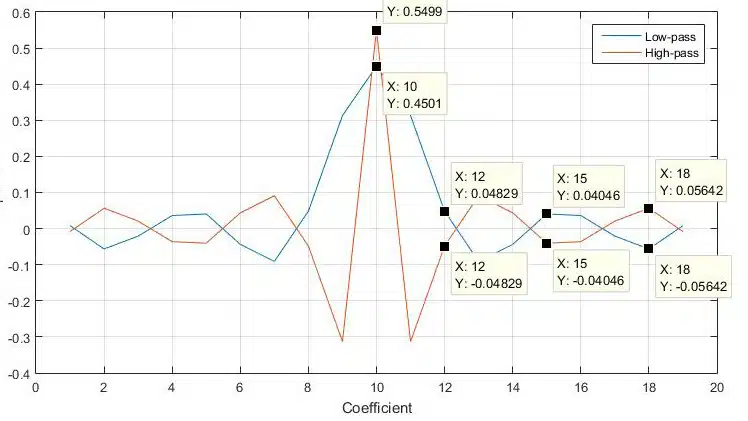
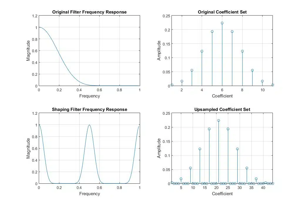
Shaping filter: a filter that has upsampled coefficient set, i.e., with zeros between the values (see Figure 11).

Image-rejection filter: this filter “interpolates” the response of the shaping filter, hence the name of the technique (it is a normal FIR filter).

What’s common between the Interpolated FIR and the Polyphase filter is the filter structure of the Shaping filter and the Transposed Polyphase, derived in the previous section. In fact, they are almost identical, except for the additional logic to multiplex the coefficient and accumulator the output.

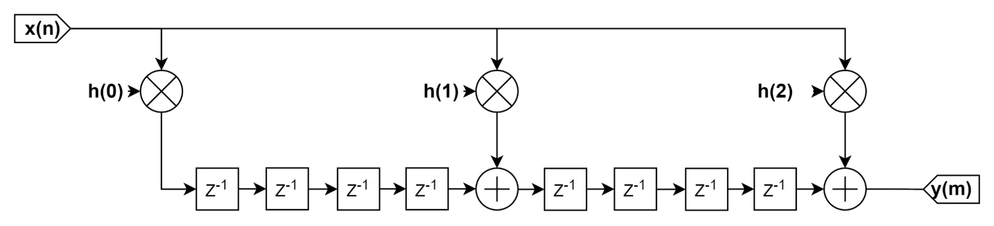
With some minor modifications, the Transposed Polyphase filter can be turned into the Shaping filter. The two filter types also share a similar design process, which is slightly more complex than the normal FIR. This, however, is outside the topic of this post.

To get a better idea, check Section 7.4 of Understanding Digital Signal Processing [4]. It describes the Shaping filter, the spectral effects of “interpolated” delay line, and how to design the image-rejection filter. It also presents the computational benefit of the IFIR, which is the main appeal behind the technique. Section 10, on the other hand, describes the sampling-rate conversion filters and how to design their frequency response.

References

• [1] Understanding Digital Signal Processing, 10 Sample Rate Conversion
• [2] Source code: DHMarinov on GitHub
• [3] Xilinx Virtex-5 FPGA XtremeDSP Design Considerations (UG193)
• [4] Understanding Digital Signal Processing, 7.4 Interpolated Lowpass FIR Filters