Part 2: Finite impulse response (FIR) filters

This article is by guest author Dimitar Marinov, whom I (Jonas) got in touch with after seeing his excellent videos about DSP filters. You can read more about Dimitry and find a link to his YouTube channel below the blog post. But first, read on to learn about FIR filter applications in FPGAs!

This article is part of a series. Click here to read Dimitar’s other articles:

Introduction

This type of digital filter is fairly easy to understand and implement as it relies exclusively on the convolution between a kernel (a set of filter coefficients) and the input. Briefly described, convolution is the operation where the respective elements of two arrays of the same size are multiplied, and all products are summed to produce one output value (see Equation 1 and Note 1).

y = \sum\limits_{k=1}^{k=K}c(k) * d(k)

Equation 1: Convolution formula

In the equation above, c is the coefficient array, d is the delay line holding the input values, and k is an array index ranging from 1 to K or 0 to K-1, depending on how the arrays are indexed.

In most applications, the input length is much bigger than the kernel length, and it can even be infinite. To keep the array size consistent, we shift the input signal along the delay line, just like cars on an assembly line, and we only use the data held by the delay elements in the filtering operation.

We refer to the number of coefficients in the kernel as the number of filter taps, Ntaps, whereas the order of the filter is Norder = Ntaps-1. By performing this operation between the two vectors, one assigns the spectral qualities of the kernel to the input signal (Note 2).

FIR Implementation

Unlike in software, where the filter has to be described in a sequential manner, in HDL the designer has the freedom to implement it either in parallel or in series.

Parallel Implementation

This approach is easy to start with as the design pretty much has to describe the signal path from the block diagram. Most commonly, the FIR filters are expressed via the Direct Form filter structure like in Figure 1. The block diagram is a direct description of the convolution process. In this case, the memory elements can be implemented as registers and the arithmetic operation via DSP slices if available.

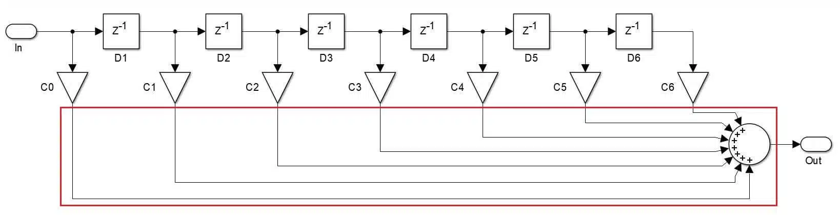
Figure 1: Block diagram of a Direct Form FIR filter — **Figure 1:** Block diagram of a Direct Form FIR filter

Summing and pipelining

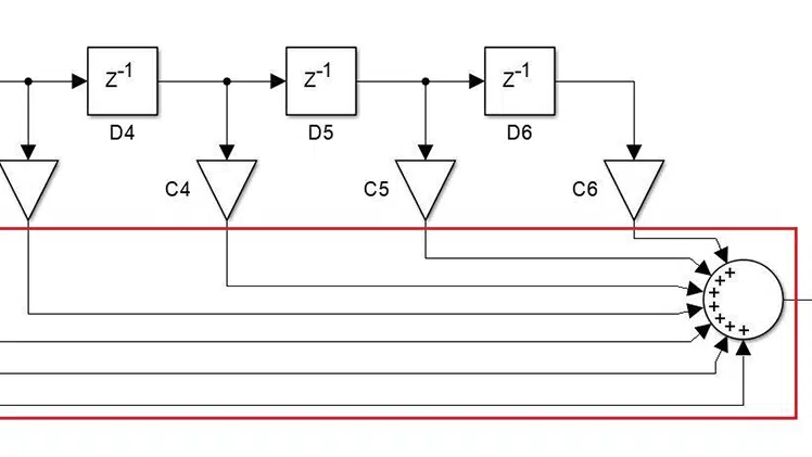
The pitfall of this filter form is the addition. Very often, the addition of 2 or more signals is described with one summing operation like in Figure 1 (the element inside the red square). Although this is feasible in HDL, it is not the most practical way to implement the operation. The logic path between the input and output register can become too long and lead to timing issues.

This is where pipelining comes in, i.e., the process of shortening the path between registers by rearranging the design or inserting registers between operations without altering the device’s functionality. Thankfully, a solution to this particular problem has been developed a long time ago (see Figure 2).

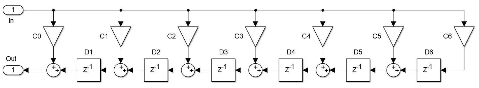
Figure 2: Transposed FIR filter — **Figure 2:** Transposed FIR filter

This filter version is way more favorable for HDL implementation – it solves the problem by breaking the addition into multiple stages separated by a register. It also simplified the input multiplication, i.e., now only the input value is involved in the multiplication. The most elegant way to implement this structure is by using For loops.

VHDL code: Parallel FIR filter

Transposed FIR Filter, where N is the number of filter taps-1 (i.e. the filter order).

--| |-----------------------------------------------------------| |
--| |-----------------------------------------------------------| |
--| |       _______           __      __      __          __    | |
--| |     /|   __  \        /|  |   /|  |   /|  \        /  |   | |
--| |    / |  |  \  \      / |  |  / |  |  / |   \      /   |   | |
--| |   |  |  |\  \  \    |  |  | |  |  | |  |    \    /    |   | |
--| |   |  |  | \  \  \   |  |  | |  |  | |  |     \  /     |   | |
--| |   |  |  |  \  \  \  |  |  |_|__|  | |  |      \/      |   | |
--| |   |  |  |   \  \  \ |  |          | |  |  |\      /|  |   | |
--| |   |  |  |   /  /  / |  |   ____   | |  |  | \    / |  |   | |
--| |   |  |  |  /  /  /  |  |  |__/ |  | |  |  |\ \  /| |  |   | |
--| |   |  |  | /  /  /   |  |  | |  |  | |  |  | \ \//| |  |   | |
--| |   |  |  |/  /  /    |  |  | |  |  | |  |  |  \|/ | |  |   | |
--| |   |  |  |__/  /     |  |  | |  |  | |  |  |      | |  |   | |
--| |   |  |_______/      |  |__| |  |__| |  |__|      | |__|   | |
--| |   |_/_______/       |_/__/  |_/__/  |_/__/       |_/__/   | |
--| |                                                           | |
--| |-----------------------------------------------------------| |
--| |=============-Developed by Dimitar H.Marinov-==============| |
--|_|-----------------------------------------------------------|_|
 
--IP: Parallel FIR Filter
--Version: V1 - Standalone 
--Fuctionality: Generic FIR filter
--IO Description
--  clk     : system clock = sampling clock
--  reset   : resets the M registes (buffers) and the P registers (delay line) of the DSP48 blocks 
--  enable  : acts as bypass switch - bypass(0), active(1) 
--  data_i  : data input (signed)
--  data_o  : data output (signed)
--
--Generics Description
--  FILTER_TAPS  : Specifies the amount of filter taps (multiplications)
--  INPUT_WIDTH  : Specifies the input width (8-25 bits)
--  COEFF_WIDTH  : Specifies the coefficient width (8-18 bits)
--  OUTPUT_WIDTH : Specifies the output width (8-43 bits)
--
--Finished on: 30.06.2019
--Notes: the DSP attribute is required to make use of the DSP slices efficiently
--------------------------------------------------------------------
--================= https://github.com/DHMarinov =================--
--------------------------------------------------------------------
 
 
 
library IEEE;
use IEEE.STD_LOGIC_1164.ALL;
use IEEE.NUMERIC_STD.ALL;
 
entity Parallel_FIR_Filter is
    Generic (
        FILTER_TAPS  : integer := 60;
        INPUT_WIDTH  : integer range 8 to 25 := 24; 
        COEFF_WIDTH  : integer range 8 to 18 := 16;
        OUTPUT_WIDTH : integer range 8 to 43 := 24    -- This should be < (Input+Coeff width-1) 
    );
    Port ( 
           clk    : in STD_LOGIC;
           reset  : in STD_LOGIC;
           enable : in STD_LOGIC;
           data_i : in STD_LOGIC_VECTOR (INPUT_WIDTH-1 downto 0);
           data_o : out STD_LOGIC_VECTOR (OUTPUT_WIDTH-1 downto 0)
           );
end Parallel_FIR_Filter;
 
architecture Behavioral of Parallel_FIR_Filter is
 
attribute use_dsp : string;
attribute use_dsp of Behavioral : architecture is "yes";
 
constant MAC_WIDTH : integer := COEFF_WIDTH+INPUT_WIDTH;
 
type input_registers is array(0 to FILTER_TAPS-1) of signed(INPUT_WIDTH-1 downto 0);
signal areg_s  : input_registers := (others=>(others=>'0'));
 
type mult_registers is array(0 to FILTER_TAPS-1) of signed(INPUT_WIDTH+COEFF_WIDTH-1 downto 0);
signal mreg_s : mult_registers := (others=>(others=>'0'));
 
type dsp_registers is array(0 to FILTER_TAPS-1) of signed(MAC_WIDTH-1 downto 0);
signal preg_s : dsp_registers := (others=>(others=>'0'));
 
signal dout_s : std_logic_vector(MAC_WIDTH-1 downto 0);
signal sign_s : signed(MAC_WIDTH-INPUT_WIDTH-COEFF_WIDTH+1 downto 0) := (others=>'0');
 
-- Chebyshev 1kH LPF, causes overflow at low freq. 
type coefficients is array (0 to 59) of signed( 15 downto 0);
signal breg_s: coefficients :=( 
 
-- 500Hz Blackman LPF
x"0000", x"0001", x"0005", x"000C", 
x"0016", x"0025", x"0037", x"004E", 
x"0069", x"008B", x"00B2", x"00E0", 
x"0114", x"014E", x"018E", x"01D3", 
x"021D", x"026A", x"02BA", x"030B", 
x"035B", x"03AA", x"03F5", x"043B", 
x"047B", x"04B2", x"04E0", x"0504", 
x"051C", x"0528", x"0528", x"051C", 
x"0504", x"04E0", x"04B2", x"047B", 
x"043B", x"03F5", x"03AA", x"035B", 
x"030B", x"02BA", x"026A", x"021D", 
x"01D3", x"018E", x"014E", x"0114", 
x"00E0", x"00B2", x"008B", x"0069", 
x"004E", x"0037", x"0025", x"0016", 
x"000C", x"0005", x"0001", x"0000");
 
 
begin 
 
 
data_o <= std_logic_vector(preg_s(0)(MAC_WIDTH-2 downto MAC_WIDTH-OUTPUT_WIDTH-1));         
       
 
process(clk)
begin
 
if rising_edge(clk) then
 
    if (reset = '1') then
        for i in 0 to FILTER_TAPS-1 loop
            areg_s(i) <=(others=> '0');
            mreg_s(i) <=(others=> '0');
            preg_s(i) <=(others=> '0');
        end loop;
 
    elsif (reset = '0') then       
        for i in 0 to FILTER_TAPS-1 loop
            areg_s(i) <= signed(data_i); 
       
            if (i < FILTER_TAPS-1) then
                mreg_s(i) <= areg_s(i)*breg_s(i);         
                preg_s(i) <= mreg_s(i) + preg_s(i+1);
                         
            elsif (i = FILTER_TAPS-1) then
                mreg_s(i) <= areg_s(i)*breg_s(i); 
                preg_s(i)<= mreg_s(i);
            end if;
        end loop; 
    end if;
     
end if;
end process;
 
end Behavioral;

Video: Efficient parallel FIR filter implementation on FPGA

Check out this video on my YouTube channel, which further explains the parallel FIR filter:

This implementation can process data as fast as the system clock can go (granted that no timing issues are present). However, since in parallel, each element from the filter block diagram requires dedicated hardware. That limits the number of filter taps the filter can use or the type of resources where the input data can be stored.

Figure 3: Parallel FIR Filter resource use — **Figure 3:** Parallel FIR Filter resource use

Serial Implementation

Parallel filters are not always the best choice – sometimes, the system clock runs way faster than the data sampling rate. In such cases, it is much better to break down the convolution process into steps and execute them one at a time. This can be implemented as a combination of a state machine, a counter and an If statement like in the following example:

VHDL code: Serial FIR filter

Direct Form FIR filter, where N is the filter order.

----------------------------------------------------------------------------------
-- Company: 
-- Engineer: 
-- 
-- Create Date: 01/15/2022 11:47:15 AM
-- Design Name: 
-- Module Name: FIR_Filter - Behavioral
-- Project Name: 
-- Target Devices: 
-- Tool Versions: 
-- Description: 
-- 
-- Dependencies: 
-- 
-- Revision:
-- Revision 0.01 - File Created
-- Additional Comments:
-- 
----------------------------------------------------------------------------------
 
 
library IEEE;
use IEEE.STD_LOGIC_1164.ALL;
 
-- Uncomment the following library declaration if using
-- arithmetic functions with Signed or Unsigned values
use IEEE.NUMERIC_STD.ALL;
 
-- Uncomment the following library declaration if instantiating
-- any Xilinx leaf cells in this code.
--library UNISIM;
--use UNISIM.VComponents.all;
 
entity FIR_Filter is
    generic(
        FILTER_TAPS : integer := 60;
        INPUT_WIDTH : integer range 8 to 32 := 16;
        COEFF_WIDTH : integer range 8 to 32 := 16;
        OUTPUT_WIDTH : integer range 8 to 32 := 16; -- This should be < (Input+Coeff width-1)
        WAITING_TIME : integer := 10;
        ADDR_WIDTH : integer range 8 to 32 := 8
    );
    Port ( 
        clk : in STD_LOGIC;
        fsclk : in STD_LOGIC;
        data_i  : in STD_LOGIC_Vector(INPUT_WIDTH-1 downto 0);
        data_o  : out STD_LOGIC_Vector(INPUT_WIDTH-1 downto 0)
    );
end FIR_Filter;
 
architecture Behavioral of FIR_Filter is
 
type input_registers is array(0 to FILTER_TAPS-1) of signed(INPUT_WIDTH-1 downto 0);
signal delay_line_s  : input_registers := (others=>(others=>'0'));
 
type coefficients is array (0 to 59) of signed( 15 downto 0);
signal coeff_s: coefficients :=( 
-- 500Hz Blackman LPF
x"0000", x"0001", x"0005", x"000C", 
x"0016", x"0025", x"0037", x"004E", 
x"0069", x"008B", x"00B2", x"00E0", 
x"0114", x"014E", x"018E", x"01D3", 
x"021D", x"026A", x"02BA", x"030B", 
x"035B", x"03AA", x"03F5", x"043B", 
x"047B", x"04B2", x"04E0", x"0504", 
x"051C", x"0528", x"0528", x"051C", 
x"0504", x"04E0", x"04B2", x"047B", 
x"043B", x"03F5", x"03AA", x"035B", 
x"030B", x"02BA", x"026A", x"021D", 
x"01D3", x"018E", x"014E", x"0114", 
x"00E0", x"00B2", x"008B", x"0069", 
x"004E", x"0037", x"0025", x"0016", 
x"000C", x"0005", x"0001", x"0000");
 
signal fsclk_q : std_logic := '0';
 
type state_machine is (idle_st, active_st);
signal state : state_machine := idle_st;
 
signal counter : integer range 0 to FILTER_TAPS-1 := FILTER_TAPS-1;
 
signal output       : signed(INPUT_WIDTH+COEFF_WIDTH-1 downto 0) := (others=>'0');
signal accumulator  : signed(INPUT_WIDTH+COEFF_WIDTH-1 downto 0) := (others=>'0');
 
begin
 
data_o <= std_logic_vector(output(INPUT_WIDTH+COEFF_WIDTH-2 downto INPUT_WIDTH+COEFF_WIDTH-OUTPUT_WIDTH-1));
 
process(clk)
 
variable sum_v : signed(INPUT_WIDTH+COEFF_WIDTH-1 downto 0) := (others=>'0');
 
begin
 
    if rising_edge(clk) then
        fsclk_q <= fsclk;
         
        case state is
        when idle_st => 
            if fsclk = '1' and fsclk_q = '0' then
                state <= active_st;
            end if;
             
        when active_st =>
            -- Counter
            if counter > 0 then
                counter <= counter - 1;
            else
                counter <= FILTER_TAPS-1;
                state <= idle_st;
            end if;
             
            -- Delay line shifting
            if counter > 0 then
                delay_line_s(counter) <= delay_line_s(counter-1);
            else
                delay_line_s(counter) <= signed(data_i);
            end if;
             
            -- MAC operations
            if counter > 0 then
                sum_v := delay_line_s(counter)*coeff_s(counter);
                accumulator <= accumulator + sum_v;    
            else
                accumulator <= (others=>'0');
                sum_v := delay_line_s(counter)*coeff_s(counter);
                output <= accumulator + sum_v;  
            end if;
             
        end case;
    end if;
 
end process;
end Behavioral;

Every time a new sample arrives, the state machine switches from idle to the active state, where the counter sweeps from N to 0. By starting the counter from n=N, the code performs the multiply-add operation on the data stored in the current N memory element and shifts the data from the N-1th element to the Nth element.

Then the counter moves to the N-1 element, and the operation repeats until the counter reaches n = 0. At n = 0, there is no more memory to read from, so the input data is assigned to the memory element of address 0, and the state goes to idle.

It is important to initialize the counter with the value of N and the state machine with the state of idle_st. In this case, the filter requires N+1 cycles to calculate the output value. This limits the filter data rate to < clock frequency / (Filter taps+1).

The biggest benefit of this implementation is the ability to reuse the hardware. In this example, the filter feeds the input and the coefficients to the same multiplier, hence reducing the arithmetic resource requirement.

Since the data is being fed sequentially, another advantage is the ability to use RAM blocks to store the data. Finally, when implementing the filter in serial, the form of the filter is far less important. In fact, the Direct Form is more suitable for serial implementation compared to the Transposed version.

Figure 4: Serial FIR Filter resource use — **Figure 4:** Serial FIR Filter resource use

Parallel vs. serial implementation

As already established, the same filter can be implemented either in parallel or in series. Both approaches have pros and cons, and these are some of the things you should consider when designing your filter:

Data rates

The parallel implementation can work at data rates equal to the system clock. For example, the DSP48 cores found in Xilinx’s 7-series can easily run at rates of +200MHz [1]. Hence the parallel option can be useful in high-speed implementations.

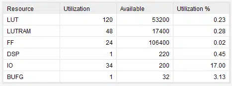
Arithmetic resources

In the parallel version, every multiply-add operation requires dedicated hardware. Therefore, designing extensive FIR filters can easily consume a large part of the available DSP resources(granted that the multipliers are implemented via the respective DSP resources and not LUTs and registers). This, however, is not the case with the serial implementation allowing to build filters of much greater order.

Memory resources

The delay elements in the parallel filter are implemented via an array of registers. This is required to accommodate the simultaneous access to the delay line. In the case of the Transposed FIR, the memory elements needed for the delay line and the pipelining are contained within the DSP slices [2], further reducing the resource requirements. On the other hand, Serial filters can use BRAMs, which makes them more flexible when it comes to resource planning.

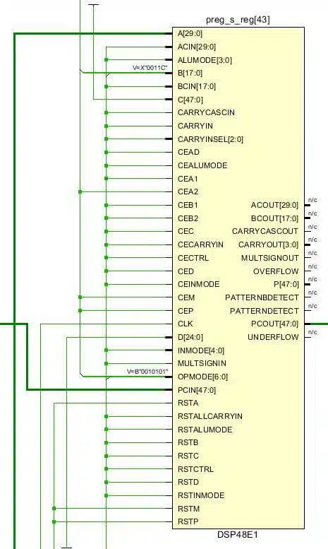
Coefficient Memory

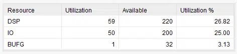
In the parallel implementation, if the coefficients are fixed, chances are the tool would not infer any registers for the coefficients as the respective multiplier inputs would be tied up to constant values (see Figure 5). However, the serial implementation does require a dedicated memory for the coefficients, which can be hosted in either a Distributed RAM or a BRAM.

Figure 5: Filter coefficients at the B port being tied up at a DSP48E1 slice — **Figure 5:** Filter coefficients at the B port being tied up at a DSP48E1 slice

Conclusion

As a designer, you don’t have to limit yourself to either parallel or serial. After all, the flexibility of the implementation target ( i.e., the FPGA or an ASIC) allows combining both methods to obtain the best result!

Part 3: FIR filter types

The follow-up article about different FIR filter types is now published. Click here to read the article:

Part 3: FIR filter types

Notes

Note 1: In theory, one of the arrays also has to be reversed before the multiplication, but this process is often skipped. This is because most filter coefficients are symmetrical around the middle value rendering the step unnecessary.
Note 2: To be precise, the convolution between two signals in the time domain is equivalent to the multiplication of their spectral content. Therefore, frequency components can be amplified or attenuated but not generated! (I think it’s the right moment to mention that the spectral properties of the filter are determined by the coefficients and not the filter structure itself.)

References

[1] Artix‐7 FPGAs Data Sheet: DC and AC Switching Characteristics
[2] 7 Series DSP48E1 Slice User Guide

3 Comments

LEE SHINHO says:

February 18, 2022 at 02:43

What it this code’s testbench code?
I can’t find that. TT

Alex says:

May 15, 2022 at 14:40

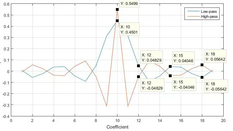
Hi, glad to find your code, it’s very helpful to understand FIR Filter implementation in VHDL. But, i have a question, how did you get the coefficient? Did you use a program like Matlab?

Thanks

Jose C. says:

July 31, 2022 at 15:45

As far as i know, the difference between serial and parallel is related to the number of samples processed at each clock cycle. Architectures you showed are pipeline or iterative.

Part 2: Finite impulse response (FIR) filters

Introduction