RC servo controller using PWM from an FPGA pin

Radio-controlled (RC) model servos are tiny actuators typically used in hobbyist model planes, cars, and boats. They allow the operator to control the vehicle via a radio link remotely. Because RC models have been around for a long time, the de-facto standard interface is pulse-width modulation (PWM), rather than a digital scheme.

Fortunately, it’s easy to implement PWM with the precise timing that an FPGA can exert on its output pins. In this article, we will create a generic servo controller that will work for any RC servo that uses PWM.

How PWM control for an RC servo works

I have already covered PWM in an earlier blog post, but we can’t use that module for controlling an RC servo. The problem is that the RC servo doesn’t expect the PWM pulses to arrive that often. It doesn’t care about the full duty cycle, only the duration of the high period.

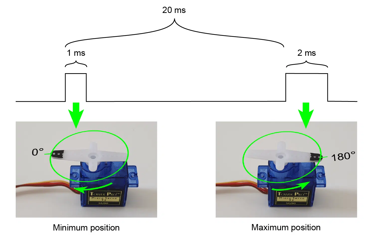
The illustration above shows how the timing of the PWM signal works.

The ideal interval between pulses is 20 ms, although it’s duration is of less importance. The 20 ms translates into a PWM frequency of 50 Hz. This means that the servo gets a new position command every 20 ms.

When a pulse arrives at the RC servo, it samples the duration of the high period. The timing is crucial because this interval translates directly to an angular position on the servo. Most servos expect to see a pulse width varying between 1 and 2 ms, but there is no set rule.

The VHDL servo controller

We will create a generic VHDL servo controller module that you can configure to work with any RC servo using PWM. To do that, we need to perform some calculations based on the value of the generic inputs.

The PWM frequencies used by RC servos are slow compared to the megahertz switching frequencies of an FPGA. Integer counting of clock cycles gives sufficient precision of the PWM pulse length. However, there will be a small rounding error unless the clock frequency matches the pulse period perfectly.

We will perform the calculations using real (floating-point) numbers, but eventually, we have to convert the results to integers. Unlike most programming languages, VHDL rounds floats to the nearest integer, but the behavior for half numbers (0.5, 1.5, etc.) is undefined. The simulator or synthesis tool may choose to round either way.

library ieee;
use ieee.std_logic_1164.all;
use ieee.numeric_std.all;
use ieee.math_real.round;

To ensure consistency across platforms, we will use the round function from the math_real library, which always rounds away from 0. The code above shows the imports in our VHDL module with the math_real library highlighted.

If you need the complete code for this project, you can download it by entering your email address in the form below. Within minutes you will receive a Zip file with the VHDL code, the ModelSim project, and the Lattice iCEcube2 project for the iCEstick FPGA board.

Servo module entity with generics

By using generic constants, we can create a module that will work for any PWM enabled RC servo. The code below shows the entity of the servo module.

The first constant is the clock frequency of the FPGA given as a real type, while pulse_hz specifies how often the PWM output shall be pulsed, and the following two constants set the pulse width in microseconds at the minimum and maximum positions. The final generic constant defines how many steps there are between the min and max position, including the endpoints.

entity servo is
  generic (
    clk_hz : real;
    pulse_hz : real; -- PWM pulse frequency
    min_pulse_us : real; -- uS pulse width at min position
    max_pulse_us : real; -- uS pulse width at max position
    step_count : positive -- Number of steps from min to max
  );
  port (
    clk : in std_logic;
    rst : in std_logic;
    position : in integer range 0 to step_count - 1;
    pwm : out std_logic
  );
end servo;

In addition to the clock and reset, the port declaration consists of a single input and a single output signal.

The position signal is the control input to the servo module. If we set it to zero, the module will produce min_pulse_us microseconds long PWM pulses. When position is at the highest value, it will produce max_pulse_us long pulses.

The pwm output is the interface to the external RC servo. It should go through an FPGA pin and connect to the “Signal” input on the servo, usually the yellow or white wire. Note that you will likely need to use a level converter. Most FPGAs use 3.3 V logic level, while most RC servos run on 5 V.

The declarative region

At the top of the servo module’s declarative region, I’m declaring a function that we will use to calculate a few constants. The cycles_per_us function, shown below, returns the closest number of clock cycles we need to count to measure us_count microseconds.

function cycles_per_us (us_count : real) return integer is
begin
  return integer(round(clk_hz / 1.0e6 * us_count));
end function;

Directly below the function, we declare the helper constants, which we will use to make the timing of the output PWM according to the generics.

First, we translate the min and max microsecond values to absolute number of clock cycles: min_count and max_count. Then, we calculate the range in microseconds between the two, from which we derive step_us, the duration difference between each linear position step. Finally, we convert the microsecond real value to a fixed number of clock periods: cycles_per_step.

constant min_count : integer := cycles_per_us(min_pulse_us);
constant max_count : integer := cycles_per_us(max_pulse_us);
constant min_max_range_us : real := max_pulse_us - min_pulse_us;
constant step_us : real := min_max_range_us / real(step_count - 1);
constant cycles_per_step : positive := cycles_per_us(step_us);

Next, we declare the PWM counter. This integer signal is a free-running counter that wraps pulse_hz times every second. That’s how we achieve the PWM frequency given in the generics. The code below shows how we calculate the number of clock cycles we have to count to, and how we use the constant to declare the range of the integer.

constant counter_max : integer := integer(round(clk_hz / pulse_hz)) - 1;
signal counter : integer range 0 to counter_max;
 
signal duty_cycle : integer range 0 to max_count;

Finally, we declare a copy of the counter named duty_cycle. This signal will determine the length of the high period on the PWM output.

Counting clock cycles

The code below shows the process that implements the free-running counter.

COUNTER_PROC : process(clk)
begin
  if rising_edge(clk) then
    if rst = '1' then
      counter <= 0;
 
    else
      if counter < counter_max then
        counter <= counter + 1;
      else
        counter <= 0;
      end if;
 
    end if;
  end if;
end process;

Unlike signed and unsigned types that are self-wrapping, we need to explicitly assign zero when the counter reaches the max value. Because we already have the max value defined in the counter_max constant, it’s easy to achieve with an If-Else construct.

PWM output process

To determine if the PWM output should be a high or low value, we compare the counter and duty_cycle signals. If the counter is less than the duty cycle, the output is a high value. Thus, the value of the duty_cycle signal controls the duration of the PWM pulse.

PWM_PROC : process(clk)
begin
  if rising_edge(clk) then
    if rst = '1' then
      pwm <= '0';
 
    else
      pwm <= '0';
 
      if counter < duty_cycle then
        pwm <= '1';
      end if;
 
    end if;
  end if;
end process;

Calculating the duty cycle

The duty cycle should never be less than min_count clock cycles because that’s the value that corresponds to the min_pulse_us generic input. Therefore, we use min_count as the reset value for the duty_cycle signal, as shown below.

DUTY_CYCLE_PROC : process(clk)
begin
  if rising_edge(clk) then
    if rst = '1' then
      duty_cycle <= min_count;
 
    else
      duty_cycle <= position * cycles_per_step + min_count;
 
    end if;
  end if;
end process;

When the module is not in reset, we calculate the duty cycle as a function of the input position. The cycles_per_step constant is an approximation, rounded to the nearest integer. Therefore, the error on this constant may be up to 0.5. When we multiply with the commanded position, the error will scale up. However, with the FPGA clock being vastly faster than the PWM frequency, it won’t be noticeable.

The servo testbench

To test the RC servo module, I’ve created a manual-check testbench that will allow us to observe the servo module’s behavior in the waveform. If you have ModelSim installed on your computer, you can download the example simulation project by entering your email address in the form below.

Simulation constants

To speed up the simulation time, we will specify a low clock frequency of 1 MHz in the testbench. I’ve also set the step count only 5, which should be sufficient for us to see the device under test (DUT) in action.

The code below shows all the simulation constants defined in the testbench.

constant clk_hz : real := 1.0e6;
constant clk_period : time := 1 sec / clk_hz;
 
constant pulse_hz : real := 50.0;
constant pulse_period : time := 1 sec / pulse_hz;
constant min_pulse_us : real := 1000.0;
constant max_pulse_us : real := 2000.0;
constant step_count : positive := 5;

DUT signals

The signals declared in the testbench match the DUT’s inputs and output. As we can see from the code below, I’ve given the clk and rst signals an initial value of ‘1’. This means that the clock will start at the high position and that the module will be in reset initially.

signal clk : std_logic := '1';
signal rst : std_logic := '1';
signal position : integer range 0 to step_count - 1;
signal pwm : std_logic;

To generate the clock signal in the testbench, I use the regular one-liner process shown below.

clk <= not clk after clk_period / 2;

DUT instantiation

Below the clock stimulus line, we proceed to instantiate the DUT. We assign the testbench constants to the generics with matching names. Furthermore, we map the DUT’s port signals to local signals in the testbench.

DUT : entity work.servo(rtl)
generic map (
  clk_hz => clk_hz,
  pulse_hz => pulse_hz,
  min_pulse_us => min_pulse_us,
  max_pulse_us => max_pulse_us,
  step_count => step_count
)
port map (
  clk => clk,
  rst => rst,
  position => position,
  pwm => pwm
);

Testbench sequencer

To provide stimuli for the DUT, we use the sequencer process shown below. First, we reset the DUT. Then, we use a For loop to iterate over all possible input positions (5 in our case). Finally, we print a message to the simulator console and end the testbench by calling the VHDL-2008 finish procedure.

SEQUENCER : process
begin
  wait for 10 * clk_period;
  rst <= '0';
 
  wait for pulse_period;
 
  for i in 0 to step_count - 1 loop
    position <= i;
    wait for pulse_period;
  end loop;
 
  report "Simulation done. Check waveform.";
  finish;
end process;

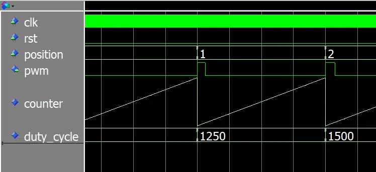
Servo simulation waveform

The waveform below shows part of the waveform that the testbench produces in ModelSim. We can see that the testbench is periodically changing the position input and that the DUT is responding by producing PWM pulses. Notice that the PWM output is high only on the lowest counter values. That’s the work of our PWM_PROC process.

If you download the project files, you should be able to reproduce the simulation by following the instructions found in the Zip file.

Example FPGA implementation

The next thing I want is to implement the design on an FPGA and let it control a real-life RC servo, the TowerPro SG90. We’ll use the Lattice iCEstick FPGA development board for that. It’s the same board as I’m using in my beginner’s VHDL course and my advanced FPGA course.

If you have the Lattice iCEstick, you can download the iCEcube2 project by using the form below.

However, the servo module can’t act alone. We need to have some supporting modules for this to work on an FPGA. At least, we need something to change the input position, and we should also have a reset module.

To make the servo motion more interesting, I’m going to use the Sine ROM module that I’ve covered in an earlier article. Together with the Counter module from the previously mentioned article, the Sine ROM will generate a smooth side-to-side movement pattern.

Read about the Sine ROM module here:
How to create a breathing LED effect using a sine wave stored in block RAM

The data flow chart below shows the submodules and how they are connected.

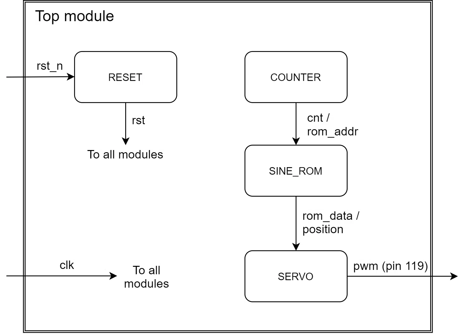
Top module entity

The top module’s entity consists of the clock and reset inputs and the PWM output, which controls the RC servo. I’ve routed the pwm signal to pin 119 on the Lattice iCE40 HX1K FPGA. That’s the leftmost pin on the leftmost header rack. The clock comes from the iCEstick’s on-board oscillator, and I’ve connected the rst signal to a pin configured with an internal pull-up resistor.

entity top is
  port (
    clk : in std_logic;
    rst_n : in std_logic; -- Pullup
    pwm : out std_logic
  );
end top; 

Signals and constants

In the top module’s declarative region, I’ve defined constants that match the Lattice iCEstick and my TowerPro SG90 servo.

Through experimenting, I found that 0.5 ms to 2.5 ms gave me the 180 degrees of movement that I wanted. Various sources on the internet suggest other values, but these are the ones that worked for me. I’m not entirely sure that I’m using a legit TowerPro SG90 servo, it might be a counterfeit.

If that’s the case, it was unintentional as I bought it from an internet seller, but it might explain the differing pulse period values. I’ve verified the durations with my oscilloscope. They are what’s written in the code that’s shown below.

constant clk_hz : real := 12.0e6; -- Lattice iCEstick clock
constant pulse_hz : real := 50.0;
constant min_pulse_us : real := 500.0; -- TowerPro SG90 values
constant max_pulse_us : real := 2500.0; -- TowerPro SG90 values
constant step_bits : positive := 8; -- 0 to 255
constant step_count : positive := 2**step_bits;

I’ve set the cnt signal for the free-running counter to be 25 bits wide, which means that it will wrap in approximately 2.8 seconds when running on the iCEstick’s 12 MHz clock.

constant cnt_bits : integer := 25;
signal cnt : unsigned(cnt_bits - 1 downto 0);

Finally, we declare the signals that will connect the top-level modules according to the data flow chart that I presented earlier. I will show how the signals below interact later in this article.

signal rst : std_logic;
signal position : integer range 0 to step_count - 1;
signal rom_addr : unsigned(step_bits - 1 downto 0);
signal rom_data : unsigned(step_bits - 1 downto 0);

Servo module instantiation

The servo module instantiation is similar to how we did it in the testbench: constant to generic, and local signal to port signal.

SERVO : entity work.servo(rtl)
generic map (
  clk_hz => clk_hz,
  pulse_hz => pulse_hz,
  min_pulse_us => min_pulse_us,
  max_pulse_us => max_pulse_us,
  step_count => step_count
)
port map (
  clk => clk,
  rst => rst,
  position => position,
  pwm => pwm
);

Self-wrapping counter instantiation

I’ve used the self-wrapping counter module in earlier articles. It’s a free-running counter that counts to counter_bits, and then goes to zero again. There’s not much to say about it, but if you want to inspect it, you can download the example project.

COUNTER : entity work.counter(rtl)
generic map (
  counter_bits => cnt_bits
)
port map (
  clk => clk,
  rst => rst,
  count_enable => '1',
  counter => cnt
);

Sine ROM instantiation

I’ve explained the Sine ROM module in detail in an earlier article. To put it short, it translates a linear number value to a full sine wave with the same min/max amplitude. The input is the addr signal, and the sine values appear on the data output.

SINE_ROM : entity work.sine_rom(rtl)
generic map (
  data_bits => step_bits,
  addr_bits => step_bits
)
port map (
  clk => clk,
  addr => rom_addr,
  data => rom_data
);

We will use the concurrent assignments shown below to connect the Counter module, the Sine ROM module, and the Servo module.

position <= to_integer(rom_data);
rom_addr <= cnt(cnt'left downto cnt'left - step_bits + 1);

The Servo module’s position input is a copy of the Sine ROM output, but we have to convert the unsigned value to an integer because they are of different types. For the ROM address input, we use the top bits of the free-running counter. By doing this, the sine wave motion cycle will complete when the cnt signal wraps, after 2.8 seconds.

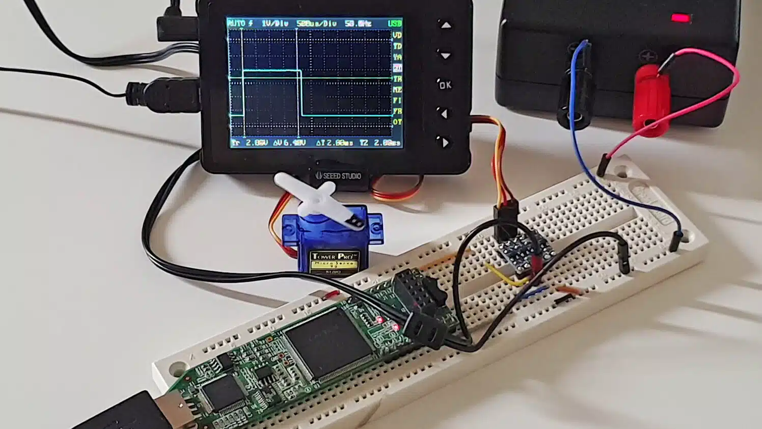
Testing on the Lattice iCEstick

I’ve hookup up the entire circuit on a breadboard, as shown by the sketch below. Because the FPGA uses 3.3 V while the servo runs at 5 V, I’ve used an external 5 V power supply and a breadboardable level shifter. Not considering the level converter, the PWM output from the FPGA pin goes directly to the “Signal” wire on the TowerPro SG90 servo.

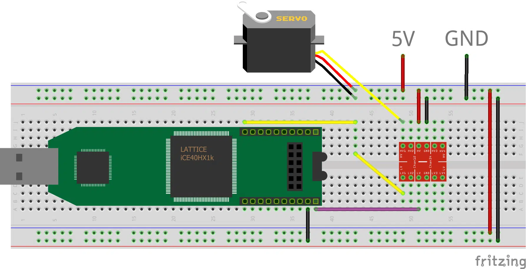
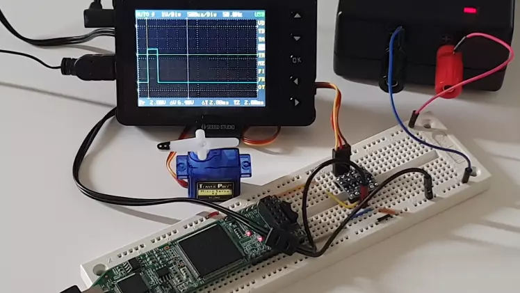
After flicking the power switch, the servo should move back and forth in a smooth 180 degrees motion, stopping slightly at the extreme positions. The video below shows my setup with the PWM signal visualized on the oscilloscope.

Final thoughts

As always, there are many ways to implement a VHDL module. But I do prefer the approach outlined in this article, using integer types as counters. All of the heavy calculations happen at compile-time, and the resulting logic is only counters, registers, and multiplexers.

The most significant hazard when dealing with 32-bit integers in VHDL is that they overflow silently in calculations. You have to check that no subexpression will overflow for any values in the expected input range. Our servo module will work for any realistic clock frequency and servo settings.

Note that this kind of PWM isn’t suitable for most applications other than RC servos. For analog power control, the duty cycle is more important than the switching frequency.

Read about analog power control using PWM here:
How to create a PWM controller in VHDL

If you want to try out the examples on your own, you can get started quickly by downloading the Zip file that I have prepared for you. Enter your email address in the form below, and you will receive everything you need to get started within minutes! The package contains the complete VHDL code, the ModelSim project with a run-script, the Lattice iCEcube2 project, and the Lattice Diamond programmer configuration file.

Let me know what you think in the comment section!